Chapter 46 Computing Monthly & Annual Turnover Rates
In this chapter, we will learn how to compute monthly and annual turnover rates.
46.1 Conceptual Overview
The turnover rate is a specific type of human resource (HR) metric, and allows us to describe past turnover in the organization relative to the total number of employees. In other words, the turnover rate is a specific type of descriptive analytics.
A monthly turnover rate refers to the turnover rate for a given month. There are various considerations one can entertain when computing monthly turnover rates, such as how broadly to define separations. That is, do we consider all forms of separations or, perhaps, just voluntary turnover. In this chapter, we will focus on a very broad and simple conceptualization and approach to computing monthly turnover rates, but please note that there are other variations. We will focus on all separations that took place in the organization (i.e., both involuntary and voluntary turnover) and coarsely account for the average number of employees in a given month. Specifically, we will use the following formula to compute a monthly turnover rate:
\(TurnoverRate_{Monthly} = \frac{Separations_{Total}}{Employees_{Average}} \times 100\)
where \(Separations_{Total}\) refers to the total number of employee separations in a given month, and \(Employees_{Average}\) refers to the average number of employees who were working in a given month. Note that we multiply the initial fraction by 100 to convert the monthly turnover rate from a proportion to a percentage.
An annual turnover rate refers to the turnover rate for a given year. Like monthly turnover rates, there are various considerations one can entertain when computing annual turnover rates, and in this tutorial we will keep things very simple by assuming that we are working with just one year’s worth of data and that we have access to separations data for all 12 months within that year. There are other ways in which we could compute annual turnover rates, but for the sake of learning, we will choose what is perhaps the most straight forward approach. Specifically, we will use the following formula to compute an annual turnover rate:
\(TurnoverRate_{Annual} = \frac{Separations_{YearSumTotal}}{Employees_{AverageAcrossMonths}} \times 100\)
where \(Separations_{YearSumTotal}\) refers to the sum total of employee separations for the year, and \(Employees_{AverageAcrossMonths}\) refers to the average number of employees who were working across the 12 months in the year. Note that we multiply the initial fraction by 100 to convert the annual turnover rate from a proportion to a percentage.
46.2 Tutorial
This chapter’s tutorial demonstrates how to compute both monthly and annual turnover rates in R.
46.2.1 Video Tutorial
As usual, you have the choice to follow along with the written tutorial in this chapter or to watch the video tutorial below.
Link to video tutorial: https://youtu.be/StdNp94V9Pk
46.2.3 Initial Steps
If you haven’t already, save the file called “turnover_rate.csv” into a folder that you will subsequently set as your working directory. Your working directory will likely be different than the one shown below (i.e., "H:/RWorkshop"). As a reminder, you can access all of the data files referenced in this book by downloading them as a compressed (zipped) folder from the my GitHub site: https://github.com/davidcaughlin/R-Tutorial-Data-Files; once you’ve followed the link to GitHub, just click “Code” (or “Download”) followed by “Download ZIP”, which will download all of the data files referenced in this book. For the sake of parsimony, I recommend downloading all of the data files into the same folder on your computer, which will allow you to set that same folder as your working directory for each of the chapters in this book.
Next, using the setwd function, set your working directory to the folder in which you saved the data file for this chapter. Alternatively, you can manually set your working directory folder in your drop-down menus by going to Session > Set Working Directory > Choose Directory…. Be sure to create a new R script file (.R) or update an existing R script file so that you can save your script and annotations. If you need refreshers on how to set your working directory and how to create and save an R script, please refer to Setting a Working Directory and Creating & Saving an R Script.
Next, read in the .csv data file called “turnover_rate.csv” using your choice of read function. In this example, I use the read_csv function from the readr package (Wickham, Hester, and Bryan 2024). If you choose to use the read_csv function, be sure that you have installed and accessed the readr package using the install.packages and library functions. Note: You don’t need to install a package every time you wish to access it; in general, I would recommend updating a package installation once ever 1-3 months. For refreshers on installing packages and reading data into R, please refer to Packages and Reading Data into R.
# Install readr package if you haven't already
# [Note: You don't need to install a package every
# time you wish to access it]
install.packages("readr")
# Access readr package
library(readr)
# Read data and name data frame (tibble) object
tr <- read_csv("turnover_rate.csv")## Rows: 12 Columns: 3
## ── Column specification ────────────────────────────────────────────────────────────────────────────────────────────────────────────
## Delimiter: ","
## dbl (3): Month, Separations, Ave_Employees
##
## ℹ Use `spec()` to retrieve the full column specification for this data.
## ℹ Specify the column types or set `show_col_types = FALSE` to quiet this message.## [1] "Month" "Separations" "Ave_Employees"## [1] 12## # A tibble: 12 × 3
## Month Separations Ave_Employees
## <dbl> <dbl> <dbl>
## 1 1 12 127
## 2 2 9 107
## 3 3 6 119
## 4 4 4 127
## 5 5 2 113
## 6 6 3 107
## 7 7 5 110
## 8 8 1 125
## 9 9 6 116
## 10 10 7 124
## 11 11 4 117
## 12 12 3 127The data frame object we named tr contains three variables: Month, Separations, and Ave_Employees. The Month variable includes 12 unique values, which correspond to the 12 months of the year, where 1 refers to January, 2 refers to February, 3 refers to March, and so on. The Separations variable includes the total number of separations (i.e., number of individuals who turned over) from the organization in a given month. The Ave_Employees variable includes the average number of employees who worked in the organization in a given month; for this example, let’s assume that the average number of employees was calculated by adding together the number of employees at the beginning of the month and the number of employees at the end of the month, and then dividing that sum by 2.
46.2.4 Compute Monthly Turnover Rates
When computing monthly turnover rates, we will create a new variable containing monthly turnover rates. To calculate the turnover rate for each month, we will use simple arithmetic by dividing the number of separations for the month divided by the average number of employees who worked in the organization that month; we can then multiply the resulting quotient by 100 to convert the proportion to a percentage. Because we are applying these arithmetic operations row by row (because in these data each row represents a unique month), our task will be relatively simple.
To illustrate how the underlying math and the logic of the operations, let’s break this process of computing monthly turnover rates into three steps. If you’re feeling confident and already understand the logic, you can skip directly to the third step, as that is what we’re building up to.
As the first step, let’s compute the monthly turnover rates as proportions and print them directly to our console. In other words, we won’t create a new variable just yet; rather, we will just peak at the monthly turnover rates (as proportions) as we get comfortable. Type in the name of the data frame object (tr) followed by the $ operator and the name of the separations variable (Separations); note that the $ operator is used to indicate which data frame object a variable belongs to. Next, type in the division symbol (/). After that, type in the name of the data frame object (tr) followed by the $ operator and the name of the average number of employees variable (Ave_Employees). Run that line of code.
# Compute monthly turnover rates (as proportions) and print to the Console
tr$Separations / tr$Ave_Employees
## [1] 0.09448819 0.08411215 0.05042017 0.03149606 0.01769912 0.02803738 0.04545455 0.00800000 0.05172414 0.05645161 0.03418803
## [12] 0.02362205In our console, we should see a vector of the monthly turnover rates as proportions.
As the second step, if we wish to view the monthly turnover rates as percentages, we just need to multiply the quotient from above by 100. In the code below, I include parentheses around the chunk of code used to compute the proportions, as I think it’s easier to conceptualize what we’re doing. That being said, because we are working with division and multiplication here, mathematical orders of operation do not require the parentheses. It’s up to you whether you decide to include them.
# Compute monthly turnover rates (as percentages) and print to the Console
(tr$Separations / tr$Ave_Employees) * 100
## [1] 9.448819 8.411215 5.042017 3.149606 1.769912 2.803738 4.545455 0.800000 5.172414 5.645161 3.418803 2.362205In our console, we should see a vector of monthly turnover rates as percentages.
As the third and final step, we will assign the vector of monthly turnover rate percentages we created above to a new variable in our data frame object. After you get the hang of computing monthly turnover rates, you can skip directly to this third step instead of building up to it using the first two steps I demonstrated above. We are simply taking the equation we used to compute monthly turnover rates as percentages and using the <- operator to assign the resulting vector of values to a new variable in our data frame object. You can call the new variable whatever you’d like, and here I call it TR_Monthly and use the $ operator to signal that I wish to attach the vector/variable to the tr data frame object we have been working with thus far.
# Compute monthly turnover rates (as percentages) and assign to variable
tr$TR_Monthly <- (tr$Separations / tr$Ave_Employees) * 100
To verify that we accomplished what we set out to do, let’s print the tr data frame object using the print function from base R.
## # A tibble: 12 × 4
##    Month Separations Ave_Employees TR_Monthly
##    <dbl>       <dbl>         <dbl>      <dbl>
##  1     1          12           127       9.45
##  2     2           9           107       8.41
##  3     3           6           119       5.04
##  4     4           4           127       3.15
##  5     5           2           113       1.77
##  6     6           3           107       2.80
##  7     7           5           110       4.55
##  8     8           1           125       0.8
##  9     9           6           116       5.17
## 10    10           7           124       5.65
## 11    11           4           117       3.42
## 12    12           3           127       2.36
We now have a new variable called TR_Monthly added to our tr data frame, and this new variable contains the monthly turnover rates as percentages. For example, we can see that for month 1 (January) the monthly turnover rate in this organization was approximately 9.45%. Often interpreting an HR metric like a turnover rate requires comparing it to other other turnover rates within the same organization (e.g., between units), to other time points (e.g., January compared to February), or to other organizations within the same industry (e.g., benchmarking).
So what can we observe or describe about these monthly turnover rates? Well, we could state the following: Monthly turnover rates were highest in the first month (January) but then declined through the fifth month (May), increasing through the seventh month (July), dropping quickly to the eighth month (August), and then increasing, plateauing, and declining in the remaining months of the year.
Optional: Given that we have access to an organization’s monthly turnover rates for an entire year, we can plot the turnover rates as a line graph to facilitate interpretation of trends. If you choose to create this optional data visualization, feel free to follow along; otherwise, you can skip down to the section called Compute Annual Turnover Rates. We will create a very simple plot using the aptly named plot function from base R. We will start with the most basic version of the line graph plot, and then add more arguments to refine it a bit.
For the first argument in our plot function, let’s specify the Month variable from the tr data frame object as our x-axis variable using the x= argument: x=tr$Month. As the second argument, let’s specify the TR_Monthly variable (we just created) from the tr data frame object as our y-axis variable using the y= argument: y=tr$TR_Monthly.
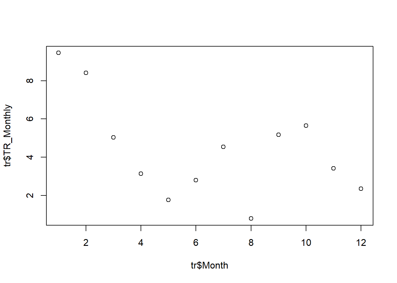
By default, the function as specified above provides us with scatter plot in our Plots window. If we wish to convert this plot to a line graph, we can add the following argument: type="l".
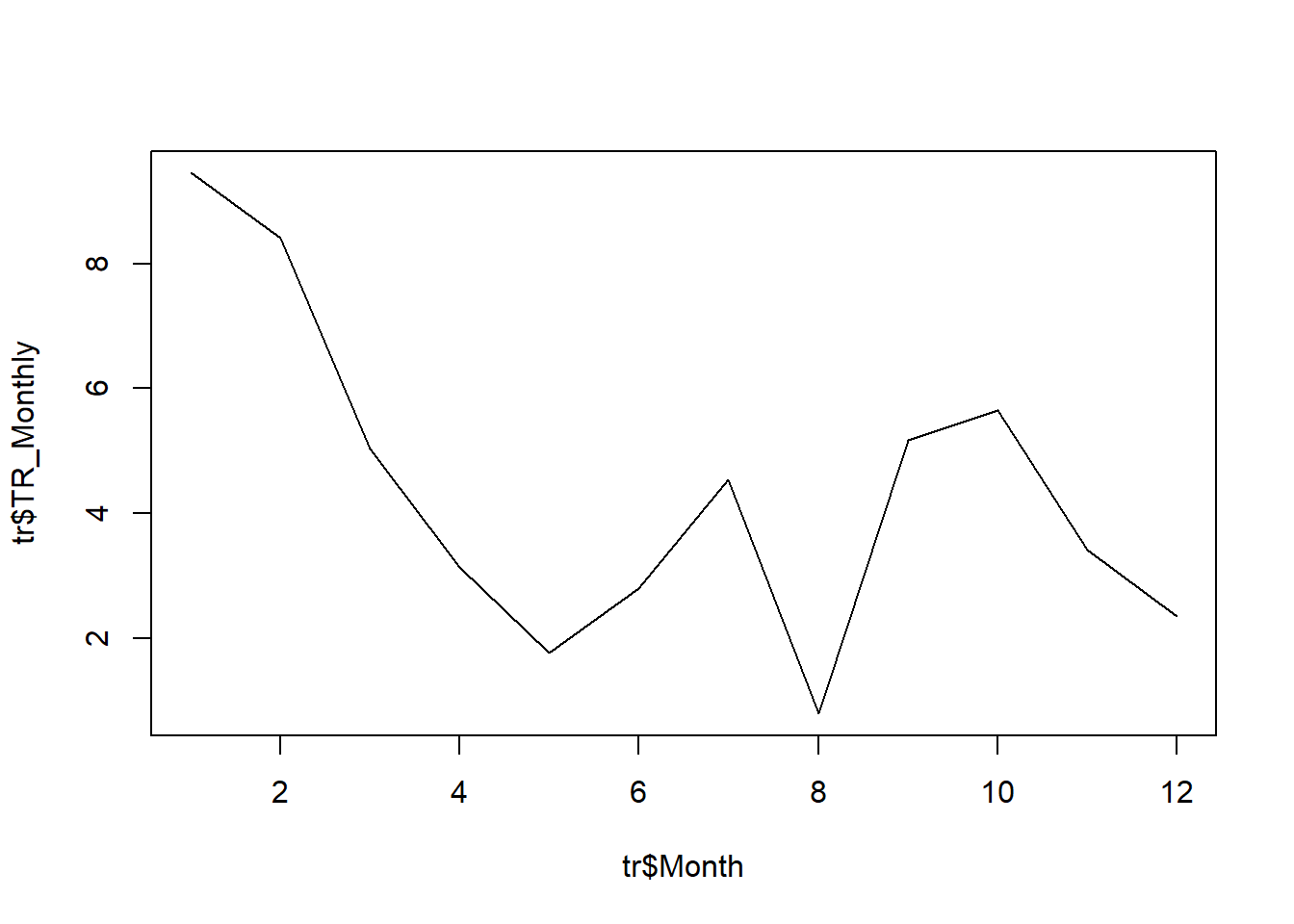
Next, we can create more meaningful x- and y-axis labels by using the xlab and ylab arguments. Note that anything we can write whatever we’d like in the quotation marks (" ").
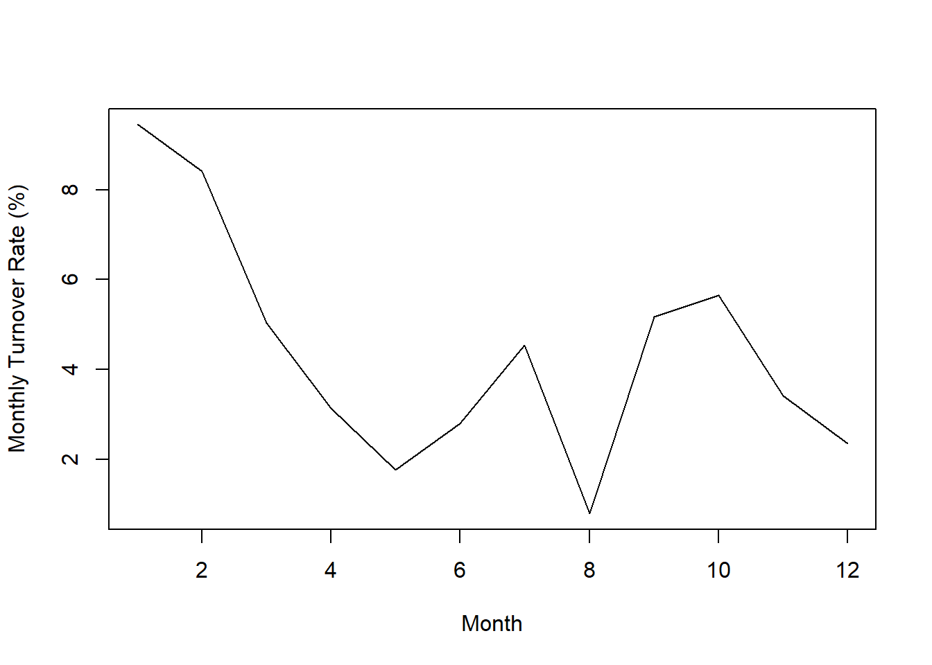
Finally, if we wish to adjust the y-axis limits, we can use the ylim argument followed by = and a vector of two values, where the first value is the lower limit of the y-axis and the second value is the upper limit. Here, we create a vector containing the lower- and upper-limits of 0 and 25 using the c (combine) function from base R.
plot(x=tr$Month, y=tr$TR_Monthly,
     type="l",
     xlab="Month",
     ylab="Monthly Turnover Rate (%)",
     ylim=c(0,25))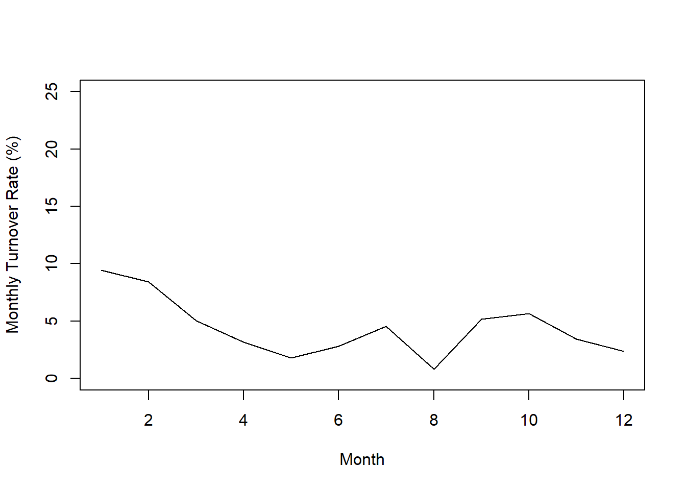
The resulting plot allows us to potentially identify and describe any trends or patterns in monthly turnover rates over the course of an entire year. Here, we can see that monthly turnover rates were highest in the first month (January) but then declined through the fifth month (May), increasing through the seventh month (July), dropping quickly to the eighth month (August), and then increasing, plateauing, and declining in the remaining months of the year. If we were to have access to data over multiple years, it’s possible we might begin to see some seasonality to the turnover rates. With access to more years worth of data, we could also build forecasting models (e.g., perform time-series analyses).
46.2.5 Compute Annual Turnover Rate
It’s time to shift gears and learn how to compute the annual turnover rate. Because we have 12 months of data from an organization for a single year, our task is relatively straight forward. When we have 12 months of turnover data for a single year, we can compute the annual turnover rate by simply summing the number of separations across the 12 months and then dividing that sum by the average number of employees across the 12 months. If we then multiply that quotient by 100, we can convert the annual turnover rate to a percentage.
Because we will need to calculate the sum and average based on values within columns, we will use the sum and mean functions, respectively, from base R. As our numerator, we type the name of the sum function; as the first argument, we enter the name of our data frame object (tr) followed by the $ operator and the name of our separations variable (Separations), and as the second argument, we enter na.rm=TRUE, which would allow us to compute the sum even if there were missing data. [You don’t technically need the na.rm=TRUE argument here given that we have complete data, but it can be good to get in the habit of including it for other applications and contexts.] As the denominator, we enter the name of the mean function; as the first argument, we enter the name of our data frame object (tr) followed by the $ operator and the name of our separations variable (Ave_Employees), and as the second argument, we enter na.rm=TRUE.
# Compute annual turnover rate (as proportion) and print to the Console
sum(tr$Separations, na.rm=TRUE) / mean(tr$Ave_Employees, na.rm=TRUE)
## [1] 0.5243129As a proportion, our annual turnover rate is approximately .5243. If we wish to convert this to a percentage, we can simply multiply our equation from above by 100.
# Compute annual turnover rate (as percentage) and print to the Console
(sum(tr$Separations, na.rm=TRUE) / mean(tr$Ave_Employees, na.rm=TRUE)) * 100
## [1] 52.43129After converting our annual turnover rate to a percentage, we see the value is approximately 52.43%.
Finally, if we wish to assign the annual turnover rate to an object that we can subsequently reference in other functions and operations, we simply apply the <- operator. Here, I’ve arbitrarily named this object TR_Annual.
# Compute annual turnover rate and assign to object
TR_Annual <- (sum(tr$Separations, na.rm=TRUE) / mean(tr$Ave_Employees, na.rm=TRUE)) * 100
We can print this object to our Console using the print function.
## [1] 52.43129Like the monthly turnover rates, an annual turnover rate is typically evaluated by comparing it to prior years, comparing between units, or comparing to industry benchmarks.