Chapter 19 Cleaning Data
In this chapter, we will learn how to clean data, such as correcting data-entry errors or removing out-of-bounds scores.
19.1 Conceptual Overview
Link to conceptual video: https://youtu.be/f8KIDg2UUKQ
Cleaning data is an essential part of the Data Management phase of the HR Analytics Project Life Cycle. When we clean data, broadly speaking, we identify, correct, or remove problematic observations, scores, or variables. More specifically, data cleaning often entails (but is not limited to):
- Identifying and correcting data-entry errors and inconsistent coding;
- Evaluating missing data and determining how to handle them;
- Flagging and correcting out-of-bounds scores for variables;
- Addressing open-ended and/or “other” responses from employee surveys;
- Flagging and potentially removing untrustworthy variables.
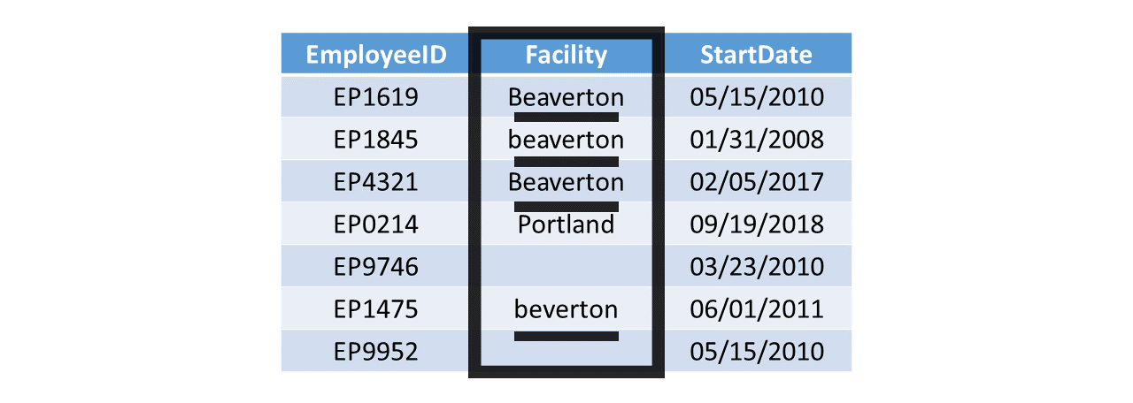
With categorical (i.e., nominal, ordinal) variables containing text values, sometimes different spellings or formatting (e.g., uppercase, lowercase) are used (mistakenly) to represent the same category. Such issues broadly fall under data-entry errors and inconsistent coding reason for data cleaning. While the human eye can usually discern what the intended category is, many software programs and programming languages will be unable to automatically or correctly determine which text values represent which category. For example, in the table below, the facility variable is categorical and contains text values meant to represent different facilities at this hypothetical organization. Human eyes can quickly pick out that there are two facility locations represented in this table: Beaverton and Portland. With that said, for the R programming language, without direction, the different spellings and different cases (i.e., lowercase vs. uppercase “B”) for the Beaverton facility (i.e., Beaverton, beaverton, beverton) will be treated as unique categories (i.e., facilities in this context). Often this is the result of data-entry errors and/or the lack of data validation. To clean the Facility variable, we could convert all instances of “beaverton” and “beverton” to “Beaverton”.
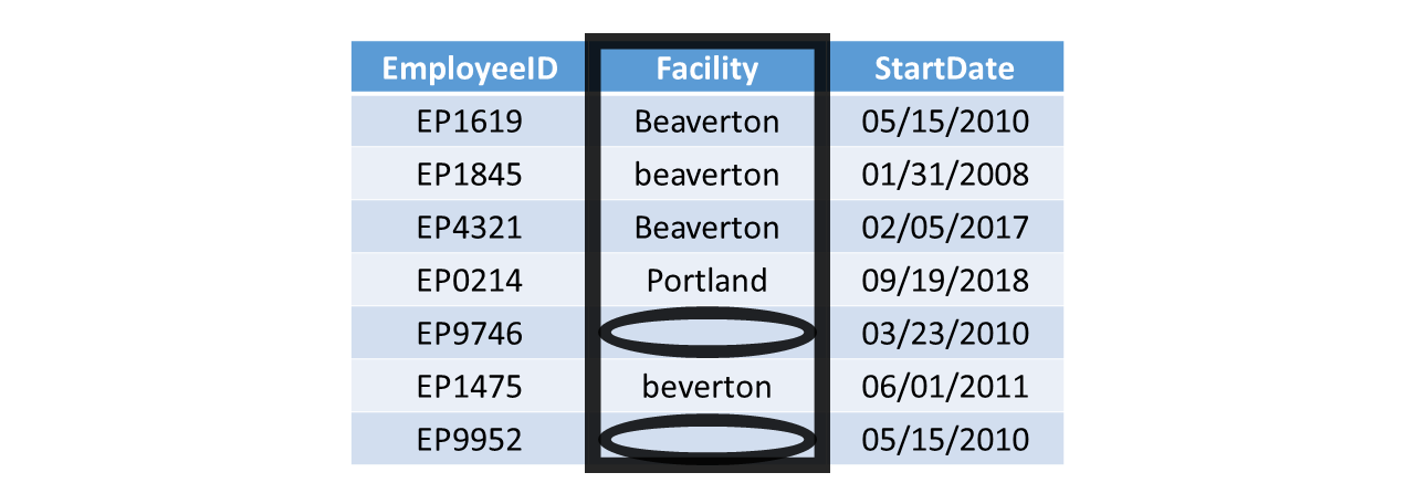
Missing data (i.e., missing scores) for certain observations (i.e., cases) should also be addressed during data cleaning. For the Facility variable in the table shown below, note how facility location data are missing for the employees with IDs EP9746 and EP9952. In this example, we could likely find other employee records or contact the employees (or their supervisors) in question to verify the facility location where these to employees work. Provided we find the facility locations for these two employees, we could then replace the missing values with the correct facility location information. In other instances, it may prove to be more difficult to replace missing data, such as when organization administers an anonymous employee survey and certain respondents have missing responses to certain questions or items. In such instances, we may decide to tolerate a small percentage of missing data (e.g., < 10%) when we go to analyze the data; however, if the percentage of missing data is sufficiently large and if we plan to analyze the data to make inferences about underlying population from which the sample data were attained, we may begin to think more seriously about whether the data are missing completely at random, missing at random, or missing at not at random. A proper discussion of missing data theory is beyond the scope of this chapter.
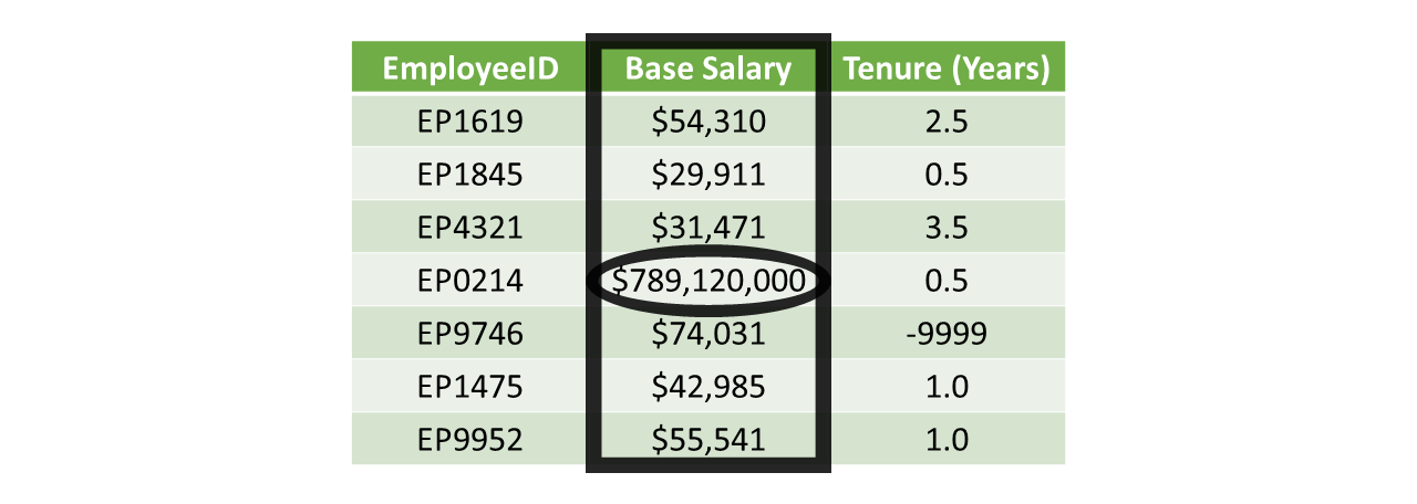
In some instances, we might encounter out-of-bounds scores, which refer to values that simply are too high or low, or that are just too unrealistic or implausible to be correct. In the table below, the Base Salary variable includes salaries that are all below 75,000 – with the notable exception of salary associated with employee ID EP0214. Let’s imagine that this table is only supposed to include data for a specific job category; knowing that, a base salary of 789,120,000 seems excessively high in a global sense and extraordinarily high in a local sense. It could be that someone entered the base salary data incorrectly for this employee, perhaps by adding four extra zeroes at the end of the actual base salary amount. In this case, we would try to find verify the correct base salary for this individual and then make the correction to the data.
If the example above seems a bit far-fetched to you, I’ll provide you with a personal example of just a single zero being mistakenly added to the end of a paycheck. After my fourth year of graduate school, I decided to teach a summer course as an adjunct faculty member, which happened to be an introductory human resource management course. During the week in which I was covering employee compensation, I received a paycheck with one extra zero added to my pay for that month, which of course increased my monthly pay 10-fold. As much as I would have enjoyed holding onto that extra money, I quickly reached out to the a representative from the university’s HR department, and the person addressed the error very quickly. At the end of the conversation, the HR representative said jokingly, “The irony is not lost on us that we made this payroll error for someone who is teaching a unit on employee compensation.”
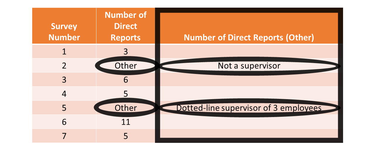
When an open-ended response or “other” response field is provided (as opposed to a close-ended response field with predetermined response options), the individual who enters the data can type in whatever they would like (in most instances) provided that they limit their response to the allotted space. This challenge crops up frequently in employee surveys, such as when employees may select an “other” response for one survey question that then branches them to a follow-up question that is open-ended. In the table below, survey respondents’ close-ended response options for the Number of Direct Reports variable include an “Other” option; respondents who responded with “Other” had an opportunity to indicate their number of direct reports using an open-ended survey question associated with the Number of Direct Reports (Other) variable. When cleaning such data, we often must determine what to do with the affect variables on a case-by-case basis. For example, the individual who responded to the survey associated with a unique identifier of 2 responded with “Not a supervisor”. If this survey was intended to acquire data from supervisors only, then we might decide to remove the row of data associated with that individual’s response, as they likely do not fit our definition of the target population.
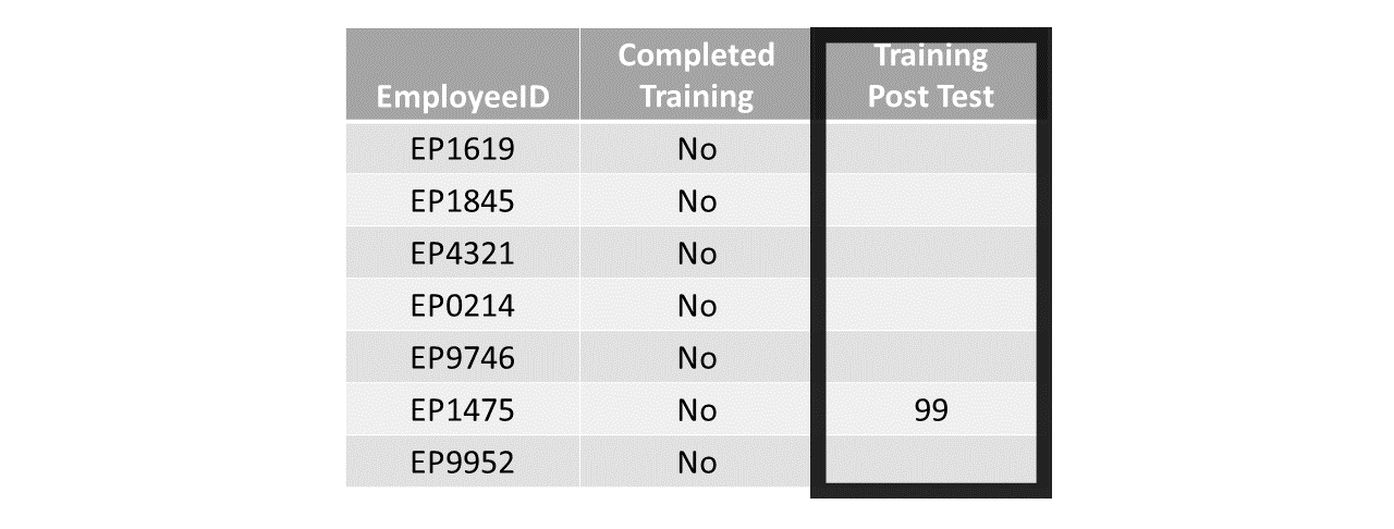
Finally, sometimes scores for a variable (or even missing scores for a variable) seem “off,” incorrect, or implausible – or in other words, untrustworthy. For example, in the table below, a variable called Training Post Test is meant to include the scores on a post-training assessment; yet, we can see that the individual with employee ID EP1475 has a score of 99 even though the adjacent variable indicates that the individual did not complete the training. Now, it’s entirely possible that this person (and others) were part of a control group (i.e., comparison group) intended to be used as part of a training evaluation design, but that then begs the question why only one individual in this table has a training post-test score. At first glance, data associated with the Training Post Test variable seem untrustworthy, and they very well may be in reality. As a next step, we would want to do some sleuthing to figure out what errors or issues may be at work in these data, and whether we should remove the potentially untrustworthy variable in question.
19.2 Tutorial
This chapter’s tutorial demonstrates different techniques for cleaning data in R.
19.2.1 Video Tutorial
As usual, you have the choice to follow along with the written tutorial in this chapter or to watch the video tutorial below.
Link to video tutorial: https://youtu.be/mGQvJ3FuNa8
19.2.2 Functions & Packages Introduced
| Function | Package |
|---|---|
View |
base R |
count |
dplyr |
str |
base R |
mutate |
dplyr |
replace |
base R |
match |
base R |
ifelse |
base R |
is.na |
base R |
toupper |
base R |
tolower |
base R |
names |
base R |
function |
base R |
clean_names |
janitor |
19.2.3 Initial Steps
If you haven’t already, save the file called “DataCleaningExample.csv” into a folder that you will subsequently set as your working directory. Your working directory will likely be different than the one shown below (i.e., "H:/RWorkshop"). As a reminder, you can access all of the data files referenced in this book by downloading them as a compressed (zipped) folder from the my GitHub site: https://github.com/davidcaughlin/R-Tutorial-Data-Files; once you’ve followed the link to GitHub, just click “Code” (or “Download”) followed by “Download ZIP”, which will download all of the data files referenced in this book. For the sake of parsimony, I recommend downloading all of the data files into the same folder on your computer, which will allow you to set that same folder as your working directory for each of the chapters in this book.
Next, using the setwd function, set your working directory to the folder in which you saved the data file for this chapter. Alternatively, you can manually set your working directory folder in your drop-down menus by going to Session > Set Working Directory > Choose Directory…. Be sure to create a new R script file (.R) or update an existing R script file so that you can save your script and annotations. If you need refreshers on how to set your working directory and how to create and save an R script, please refer to Setting a Working Directory and Creating & Saving an R Script.
Next, read in the .csv data file called “DataCleaningExample.csv” using your choice of read function. In this example, I use the read_csv function from the readr package (Wickham, Hester, and Bryan 2024). If you choose to use the read_csv function, be sure that you have installed and accessed the readr package using the install.packages and library functions. Note: You don’t need to install a package every time you wish to access it; in general, I would recommend updating a package installation once ever 1-3 months. For refreshers on installing packages and reading data into R, please refer to Packages and Reading Data into R.
# Install readr package if you haven't already
# [Note: You don't need to install a package every
# time you wish to access it]
install.packages("readr")
# Access readr package
library(readr)
# Read data and name data frame (tibble) object
df <- read_csv("DataCleaningExample.csv")## Rows: 10 Columns: 6
## ── Column specification ────────────────────────────────────────────────────────────────────────────────────────────────────────────
## Delimiter: ","
## chr (3): EmpID, Facility, OnboardingCompleted
## dbl (2): JobLevel, Org_Tenure_Yrs
## date (1): StartDate
##
## ℹ Use `spec()` to retrieve the full column specification for this data.
## ℹ Specify the column types or set `show_col_types = FALSE` to quiet this message.## [1] "EmpID" "Facility" "JobLevel" "StartDate" "Org_Tenure_Yrs"
## [6] "OnboardingCompleted"## # A tibble: 10 × 6
## EmpID Facility JobLevel StartDate Org_Tenure_Yrs OnboardingCompleted
## <chr> <chr> <dbl> <date> <dbl> <chr>
## 1 EP1201 Beaverton 1 2010-05-05 8.6 No
## 2 EP1202 beaverton 1 2008-01-31 10.9 No
## 3 EP1203 Beaverton -9999 2017-02-05 1.9 No
## 4 EP1204 Portland 5 2018-09-19 0.3 No
## 5 EP1205 <NA> 2 2018-09-19 0.3 No
## 6 EP1206 Beaverton 1 2010-03-23 8.8 No
## 7 EP1207 beverton 1 2011-06-01 7.6 No
## 8 EP1208 Portland 4 2010-05-15 8.6 No
## 9 EP1209 Portland 3 2011-04-29 7.7 No
## 10 EP1210 Beaverton 11 2012-07-11 6.5 NoNote in the data frame that the EmpID field/variable is a unique identifier variable, which means that each case/observation has a unique value on this field/variable. This will become useful later on in this tutorial when we replace values on variables for specific cases.
19.2.4 Review Data
There are different tools and techniques we can use to review the cleanliness or integrity of the available data. Often, it’s a good idea to give the data a once over with what I refer to as the “ocular test,” which simply means to scan the raw data using your eyes. The ocular test can give you an idea of the types of data cleaning issues you’ll need to address. The View function from base R is a great tool for this, as it allows you to look at the data frame object in a viewer tab, and using the arrows at the top of each column, you can sort each field (i.e., variable) manually.
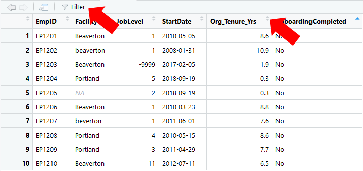
View function from base R.In addition, applying the count function from the dplyr package (Wickham et al. 2023) can provide us with an understanding of the values (or lack thereof) associated with each variable in your data frame object. The count function groups and tallies the number of observations (i.e., frequencies) by value/level within a variable. Using this function we can (hopefully) identify any values that might be considered “out of bounds” or erroneous. Because the count function comes from the dplyr package, if you haven’t already, install and access the dplyr package using the install.packages and library functions, respectively.
We can achieve the same output with and without the use of the pipe (%>%) operator because the dplyr package is built upon the magrittr (Bache and Wickham 2022) package. For more information on the pipe operator, check out this link: https://r4ds.had.co.nz/pipes.html. If you don’t want to use the pipe operator with the dplyr functions, just skip down below to see how to specify the function without using pipes.
Using the pipe (%>%) operator, first, type the name of the data frame object to which a variable belongs (e.g., df). Second, type the %>% operator. Third, type the name of the count function, and within the parentheses, enter the exact name of the variable (e.g., Facility) as the sole argument.
## # A tibble: 5 × 2
##   Facility      n
##   <chr>     <int>
## 1 Beaverton     4
## 2 Portland      3
## 3 beaverton     1
## 4 beverton      1
## 5 <NA>          1
Note that the output yields a table object (or more specifically a “tibble”, which is used in the tidyverse collection of functions). There are two columns: (a) the variable name, below which appears all values/levels of that variable, and (b) the n column, which displays the number of cases/observations associated with each value/level of the variable in question. As you can see, there appear to be some errors. Perhaps the database used to gather these data lacked data validation rules for certain variables, which allowed users to enter different spellings or formatting of the same value/level of the variables. For example, the Beaverton facility is spelled/formatted in three ways: Beaverton, beaverton, and beverton. Because R is case sensitive, Beaverton and beaverton are treated as to distinct levels/values of the Facility variable. Further, beverton is a misspelling of Beaverton and lacks the capital B. Finally, note that there is one NA value, which indicates that someone forgot to enter the name of the facility where that employee works. Clearly, we need to correct these errors and clean up the data residing within this variable; later in the tutorial, you will learn how to correct/replace these values in the R environment.
To perform the operation above without the pipe (%>%) operator,type the name of the count function, and within the parentheses, type the name of the data frame object (df) as the first argument, followed by a comma. As the second argument, type the exact name of the variable (e.g., Facility).
## # A tibble: 5 × 2
##   Facility      n
##   <chr>     <int>
## 1 Beaverton     4
## 2 Portland      3
## 3 beaverton     1
## 4 beverton      1
## 5 <NA>          1
As you can see, the output is the same with and without the use of the pipe (%>%) operator.
Now let’s apply the count function to the JobLevel variable. To save space, I only show how to do this using the pipe operator (%>%). All we need to do is replace Facility with JobLevel in the syntax/code we wrote previously.
## # A tibble: 7 × 2
##   JobLevel     n
##      <dbl> <int>
## 1    -9999     1
## 2        1     4
## 3        2     1
## 4        3     1
## 5        4     1
## 6        5     1
## 7       11     1
For the sake of this example, let’s assume that the company has only five job levels (1 = lowest, 5 = highest). In the output, it is apparent that there are two out-of-bounds values: -9999 and 11. Rather than leave cell blank when entering data, some people prefer to use extreme negative values, such as -9999, to flag missing data, and let’s assume that is the case in this example. A potential issue with this approach to coding missing data is that R assumes -9999 is a real value, and in R, NA is often used to indicate missing data to avoid this issue. Regarding the 11 value, it is likely that someone made an error when entering the data value in the database by typing 1 twice by mistake; let’s assume that we verified that this was the case and that 11 should be replaced with 1.
Lastly, let’s apply the count function to the OnboardingCompleted variable.
## # A tibble: 1 × 2
##   OnboardingCompleted     n
##   <chr>               <int>
## 1 No                     10
In this example, employees either completed (Yes) or did not complete (No) the onboarding for new employees. As you can see in the output, there are no missing data (i.e., all 10 cases have a value); however, note that every single case/observation (i.e., employee) has the value No when in actuality (let’s assume) every single case/observation should have the value Yes because we learned that every single employee in this data frame completed the onboarding program.
In the next section, you will learn how to clean the “dirty” data we identified within the Facility, JobLevel, and OnboardingCompleted variables.
19.2.5 Clean Data
As is often the case in R (and in life), there are multiple approaches to cleaning data. I demonstrate two approaches in this tutorial: (a) replacing a value for specific cases/observations with the correct value and (b) replacing a specific value for all cases that have the same value on that variable. Both approaches can come in handy given the particular data-cleaning circumstance you are facing.
19.2.5.1 Replace a Specific Value for a Specific Case
To begin, let’s replace a specific value for a specific case/observation. To do so, we’ll apply three functions: mutate from the dplyr package and replace and match from base R. If you haven’t already, be sure that you have installed and accessed the dplyr package using the install.packages and library functions, respectively. Using the pipe (%>%) operator, we can replace a specific value for a specific case by:
- Type the name of a new data frame object, as it is generally a good practice to preserve the original data frame you read in earlier; here, I arbitrarily name the new data frame object
newdf1. - Type the
<-operator to the right of the new data frame object so that the results of the subsequent operations can be assigned to the new object. - Type the name of the original data frame object (
df), followed by the pipe (%>%) operator. - Type the name of the
mutatefunction. Within themutatefunction parentheses, provide the name of an existing or new variable; in this case, we will overwrite the existingFacilityvariable by typing the same variable name. Next, enter the=operator to the right of themutatefunction to specify how values for theFacilityvariable will be determined. - Type the name of the
replacefunction, which is a function that allows one to replace values in specific location within a vector or data frame. Within thereplacefunction parentheses, as the first argument, type the name of the variable for which you wish to replace specific values (Facility). As the second argument, type the name of thematchfunction, which is a function that allows us to find matched value(s) within a variable (i.e., vector); s the first argument within thematchfunction, enter the value you wish to find a match for (“EP1202”), and as the second argument, enter the name of the variable (EmpID) to which that value belongs. Essentially, thismatchfunction and its two arguments will instruct R to identify the case in whichEmpID(variable name) is equal to “EP1202”. Because the variableEmpIDis of type character (chr), the value identified from that variable should be placed in quotation marks (" "); if the variable were of type numeric, you would not include the quotation marks (" "), and as shown below, thestr(structure) function can be used to identify the variable type for the variables within a data frame object (e.g.,df); as the final (third) argument within thereplacefunction, enter the new value (e.g., “Beaverton”) that you would like to replace the existing value with for the particular case you identified.
## spc_tbl_ [10 × 6] (S3: spec_tbl_df/tbl_df/tbl/data.frame)
##  $ EmpID              : chr [1:10] "EP1201" "EP1202" "EP1203" "EP1204" ...
##  $ Facility           : chr [1:10] "Beaverton" "beaverton" "Beaverton" "Portland" ...
##  $ JobLevel           : num [1:10] 1 1 -9999 5 2 ...
##  $ StartDate          : Date[1:10], format: "2010-05-05" "2008-01-31" "2017-02-05" "2018-09-19" ...
##  $ Org_Tenure_Yrs     : num [1:10] 8.6 10.9 1.9 0.3 0.3 8.8 7.6 8.6 7.7 6.5
##  $ OnboardingCompleted: chr [1:10] "No" "No" "No" "No" ...
##  - attr(*, "spec")=
##   .. cols(
##   ..   EmpID = col_character(),
##   ..   Facility = col_character(),
##   ..   JobLevel = col_double(),
##   ..   StartDate = col_date(format = ""),
##   ..   Org_Tenure_Yrs = col_double(),
##   ..   OnboardingCompleted = col_character()
##   .. )
##  - attr(*, "problems")=<externalptr>
# For EmpID equal to EP1202, replace "beaverton" with "Beaverton" using pipe
newdf1 <- df %>%
mutate(Facility = replace(Facility,
match("EP1202", EmpID),
"Beaverton"))
# Print new data frame object
print(newdf1)## # A tibble: 10 × 6
## EmpID Facility JobLevel StartDate Org_Tenure_Yrs OnboardingCompleted
## <chr> <chr> <dbl> <date> <dbl> <chr>
## 1 EP1201 Beaverton 1 2010-05-05 8.6 No
## 2 EP1202 Beaverton 1 2008-01-31 10.9 No
## 3 EP1203 Beaverton -9999 2017-02-05 1.9 No
## 4 EP1204 Portland 5 2018-09-19 0.3 No
## 5 EP1205 <NA> 2 2018-09-19 0.3 No
## 6 EP1206 Beaverton 1 2010-03-23 8.8 No
## 7 EP1207 beverton 1 2011-06-01 7.6 No
## 8 EP1208 Portland 4 2010-05-15 8.6 No
## 9 EP1209 Portland 3 2011-04-29 7.7 No
## 10 EP1210 Beaverton 11 2012-07-11 6.5 NoIn the new data frame object (newdf1), you should now see that “beaverton” has been replaced with “Beaverton” for the case in which EmpID is equal to “EP1202”. Assuming you save your script as an R script file (.R), you will have a paper trail that shows that you replaced an existing value with a new (correct) value.
To apply the mutate function without a pipe (%>%) operator, we simply remove the pipe (%>%) operator and enter the name of our original data frame object (df) as the first argument of the mutate function.
# For EmpID equal to EP1202, replace "beaverton" with "Beaverton" without using pipe
newdf1 <- mutate(df,
                 Facility = replace(Facility,
                                    match("EP1202",EmpID),
                                    "Beaverton"))

# Print new data frame object
print(newdf1)
## # A tibble: 10 × 6
## EmpID Facility JobLevel StartDate Org_Tenure_Yrs OnboardingCompleted
## <chr> <chr> <dbl> <date> <dbl> <chr>
## 1 EP1201 Beaverton 1 2010-05-05 8.6 No
## 2 EP1202 Beaverton 1 2008-01-31 10.9 No
## 3 EP1203 Beaverton -9999 2017-02-05 1.9 No
## 4 EP1204 Portland 5 2018-09-19 0.3 No
## 5 EP1205 <NA> 2 2018-09-19 0.3 No
## 6 EP1206 Beaverton 1 2010-03-23 8.8 No
## 7 EP1207 beverton 1 2011-06-01 7.6 No
## 8 EP1208 Portland 4 2010-05-15 8.6 No
## 9 EP1209 Portland 3 2011-04-29 7.7 No
## 10 EP1210 Beaverton 11 2012-07-11 6.5 NoNow let’s take the newdf1 data frame object we just created and replace “beverton” with “Beaverton” for the case in which the EmpID variable value is equal to “EP1207”. All we need to do in this instance is to (a) swap out df with newdf1 as the original data frame name and (b) swap out “EP1202” with “EP1207” from the previous piped code we wrote.
# For EmpID equal to EP1207, replace "beverton" with "Beaverton" using pipe
newdf1 <- newdf1 %>%
  mutate(Facility = replace(Facility,
                            match("EP1207", EmpID),
                            "Beaverton"))

# Print new data frame object
print(newdf1)
## # A tibble: 10 × 6
## EmpID Facility JobLevel StartDate Org_Tenure_Yrs OnboardingCompleted
## <chr> <chr> <dbl> <date> <dbl> <chr>
## 1 EP1201 Beaverton 1 2010-05-05 8.6 No
## 2 EP1202 Beaverton 1 2008-01-31 10.9 No
## 3 EP1203 Beaverton -9999 2017-02-05 1.9 No
## 4 EP1204 Portland 5 2018-09-19 0.3 No
## 5 EP1205 <NA> 2 2018-09-19 0.3 No
## 6 EP1206 Beaverton 1 2010-03-23 8.8 No
## 7 EP1207 Beaverton 1 2011-06-01 7.6 No
## 8 EP1208 Portland 4 2010-05-15 8.6 No
## 9 EP1209 Portland 3 2011-04-29 7.7 No
## 10 EP1210 Beaverton 11 2012-07-11 6.5 NoLet’s assume that after looking through other organizational records we found that the employee with EmpID equal to “EP1205” works at the “Portland” facility. Accordingly, we want to replace the NA value for the Facility variable for that employee with “Portland”. When adapting the previous script/code, all we need to do is replace “EP1207” with “EP1205” and “Beaverton” with “Portland”.
# For EmpID equal to EP1205, replace NA with "Portland" using pipe
newdf1 <- newdf1 %>%
  mutate(Facility = replace(Facility,
                            match("EP1205", EmpID),
                            "Portland"))

# Print new data frame object
print(newdf1)
## # A tibble: 10 × 6
## EmpID Facility JobLevel StartDate Org_Tenure_Yrs OnboardingCompleted
## <chr> <chr> <dbl> <date> <dbl> <chr>
## 1 EP1201 Beaverton 1 2010-05-05 8.6 No
## 2 EP1202 Beaverton 1 2008-01-31 10.9 No
## 3 EP1203 Beaverton -9999 2017-02-05 1.9 No
## 4 EP1204 Portland 5 2018-09-19 0.3 No
## 5 EP1205 Portland 2 2018-09-19 0.3 No
## 6 EP1206 Beaverton 1 2010-03-23 8.8 No
## 7 EP1207 Beaverton 1 2011-06-01 7.6 No
## 8 EP1208 Portland 4 2010-05-15 8.6 No
## 9 EP1209 Portland 3 2011-04-29 7.7 No
## 10 EP1210 Beaverton 11 2012-07-11 6.5 NoNow that the Facility variable has been cleaned, let’s move on to the JobLevel variable. If you recall, in the previous section, we determined that there were two problematic values for two cases: -9999 (associated with EmpID equal to “1203”) and 11 (associated with EmpID equal to “1210”). We decided that -9999 should be replace with NA because it represents a missing value, and 11 should be replaced with 1 because it represents a data entry error. Check out the script/code below to see how these replacements were handled. Also, note that because the JobLevel variable is of type numeric, we don’t put the replacement values of NA and 1 in direct quotations.
# For EmpID equal to EP1203, replace -9999 with NA using pipe
newdf1 <- newdf1 %>%
  mutate(JobLevel = replace(JobLevel,
                            match("EP1203", EmpID),
                            NA))

# Print new data frame object
print(newdf1)
## # A tibble: 10 × 6
## EmpID Facility JobLevel StartDate Org_Tenure_Yrs OnboardingCompleted
## <chr> <chr> <dbl> <date> <dbl> <chr>
## 1 EP1201 Beaverton 1 2010-05-05 8.6 No
## 2 EP1202 Beaverton 1 2008-01-31 10.9 No
## 3 EP1203 Beaverton NA 2017-02-05 1.9 No
## 4 EP1204 Portland 5 2018-09-19 0.3 No
## 5 EP1205 Portland 2 2018-09-19 0.3 No
## 6 EP1206 Beaverton 1 2010-03-23 8.8 No
## 7 EP1207 Beaverton 1 2011-06-01 7.6 No
## 8 EP1208 Portland 4 2010-05-15 8.6 No
## 9 EP1209 Portland 3 2011-04-29 7.7 No
## 10 EP1210 Beaverton 11 2012-07-11 6.5 No# For EmpID equal to EP1210, replace 11 with 1 using pipe
newdf1 <- newdf1 %>%
mutate(JobLevel = replace(JobLevel,
match("EP1210", EmpID),
1))
# Print new data frame object
print(newdf1)## # A tibble: 10 × 6
## EmpID Facility JobLevel StartDate Org_Tenure_Yrs OnboardingCompleted
## <chr> <chr> <dbl> <date> <dbl> <chr>
## 1 EP1201 Beaverton 1 2010-05-05 8.6 No
## 2 EP1202 Beaverton 1 2008-01-31 10.9 No
## 3 EP1203 Beaverton NA 2017-02-05 1.9 No
## 4 EP1204 Portland 5 2018-09-19 0.3 No
## 5 EP1205 Portland 2 2018-09-19 0.3 No
## 6 EP1206 Beaverton 1 2010-03-23 8.8 No
## 7 EP1207 Beaverton 1 2011-06-01 7.6 No
## 8 EP1208 Portland 4 2010-05-15 8.6 No
## 9 EP1209 Portland 3 2011-04-29 7.7 No
## 10 EP1210 Beaverton 1 2012-07-11 6.5 NoFinally, let’s assume that for the OnboardingCompleted variable, two of the cases have values that should in fact be NA (missing). Specifically, because the hypothetical onboarding program takes 1.0 year to complete, the two employees (cases) with Org_Tenure_Yrs (organizational tenure in years) equal to 0.3 have not worked in the company long enough to have completed the 1-year-long onboarding program. Consequently, we decide that it is not appropriate to put “No” or “Yes” for these two employees, which means treating those values as missing (NA) would be most appropriate. The two employees in question have EmpID variable values of “EP1204” and “EP1205”. Note that we can enter NA as the final argument within the replace function parentheses, just as we would with an actual value. Check out the script/code below to see how we replace 0.3 with NA on the OnboardingCompleted variable for the cases with the EmpID unique identifier variable equal to “EP1204” and “EP1205”.
# For EmpID equal to EP1204, replace 0.3 with NA using pipe
newdf1 <- newdf1 %>%
  mutate(OnboardingCompleted = replace(OnboardingCompleted,
                                       match("EP1204", EmpID),
                                       NA))

# For EmpID equal to EP1205, replace 0.3 with NA using pipe
newdf1 <- newdf1 %>%
  mutate(OnboardingCompleted = replace(OnboardingCompleted,
                                       match("EP1205", EmpID),
                                       NA))

# Print new data frame object
print(newdf1)
## # A tibble: 10 × 6
## EmpID Facility JobLevel StartDate Org_Tenure_Yrs OnboardingCompleted
## <chr> <chr> <dbl> <date> <dbl> <chr>
## 1 EP1201 Beaverton 1 2010-05-05 8.6 No
## 2 EP1202 Beaverton 1 2008-01-31 10.9 No
## 3 EP1203 Beaverton NA 2017-02-05 1.9 No
## 4 EP1204 Portland 5 2018-09-19 0.3 <NA>
## 5 EP1205 Portland 2 2018-09-19 0.3 <NA>
## 6 EP1206 Beaverton 1 2010-03-23 8.8 No
## 7 EP1207 Beaverton 1 2011-06-01 7.6 No
## 8 EP1208 Portland 4 2010-05-15 8.6 No
## 9 EP1209 Portland 3 2011-04-29 7.7 No
## 10 EP1210 Beaverton 1 2012-07-11 6.5 No19.2.5.2 Replace a Specific Value for All Cases with a Particular Value
If you need to systematically clean multiple values for a given variable, there is another approach that is more efficient. Note that this approach is only appropriate if you have identified that the values in question all need to be changed to the same value. For the sake of this example, let’s pretend that all of the “No” values for the OnboardingCompleted variable were entered incorrectly. Instead of “No”, the value should be “Yes” for each of these cases. First, you will learn how to replace these values in one fell swoop using the mutate function from the dplyr package and the ifelse function from base R. Second, you will learn how to do the same thing without the use of a specific function.
Let’s start with the first approach, which involves the mutate and ifelse functions. Using the pipe (%>%) operator, we can do the following:
- Type the name of a new data frame object; here, I use the same name as the original name to overwrite the existing data frame object called
newdf1. - Type the
<-operator to the right of the new data frame object so that the results of the subsequent operations can be assigned to the new object. - Type the name of the original data frame object (
newdf1), followed by the pipe (%>%) operator. - Type the name of the
mutatefunction. Within themutatefunction parentheses, provide the name of an existing or a new variable; in this case, we will overwrite the existingOnboardingCompletedvariable by typing the same name as the existing variable. To the right of themutatefunction, type the=operator to specify how values for theOnboardingCompletedvariable will be determined. - Type the name of the
ifelsefunction, which is a function that can be used for conditional value (element) selection (identification) and replacement. As the first argument, type a conditional statement for the variable whose values you wish to replace; because we wish to replace all “No” values with “Yes” for theOnboardingCompletedvariable, we’ll specify the conditional statement asOnboardingCompleted=="No"; for a review of the different logical operators, please refer to the chapter called Filtering Data. As the second argument in theifelsefunction, type the replacement value when the aforementioned conditional statement is true for a given value of theOnboardingCompletedvariable, which is “Yes” in this example. Because theOnboardingCompletedvariable is of type character, this value needs to be in quotation marks (" "). As the final argument function, instruct theifelsefunction what the replacement value should be when the aforementioned conditional statement is false, which in this; in this example, we will replace all other values with the existing values of theOnboardingCompletedvariable, and thus we’ll enter that variable name as the third argument.
# For OnboardingCompleted variable, replace "No" values with "Yes" using pipe
newdf1 <- newdf1 %>%
  mutate(OnboardingCompleted = ifelse(OnboardingCompleted=="No",
                                      "Yes",
                                      OnboardingCompleted))

# Print new data frame object
print(newdf1)
## # A tibble: 10 × 6
## EmpID Facility JobLevel StartDate Org_Tenure_Yrs OnboardingCompleted
## <chr> <chr> <dbl> <date> <dbl> <chr>
## 1 EP1201 Beaverton 1 2010-05-05 8.6 Yes
## 2 EP1202 Beaverton 1 2008-01-31 10.9 Yes
## 3 EP1203 Beaverton NA 2017-02-05 1.9 Yes
## 4 EP1204 Portland 5 2018-09-19 0.3 <NA>
## 5 EP1205 Portland 2 2018-09-19 0.3 <NA>
## 6 EP1206 Beaverton 1 2010-03-23 8.8 Yes
## 7 EP1207 Beaverton 1 2011-06-01 7.6 Yes
## 8 EP1208 Portland 4 2010-05-15 8.6 Yes
## 9 EP1209 Portland 3 2011-04-29 7.7 Yes
## 10 EP1210 Beaverton 1 2012-07-11 6.5 YesNow let’s pretend that we wish to convert the “Yes” values for the OnboardingCompleted variable with the numeric value of 1. The format of the code remains virtually the same, except that we change the conditional statement to OnboardingCompleted=="Yes" as the first argument in the ifelse function, and in the second argument, we change the replacement value to 1.
# For OnboardingCompleted variable, replace "Yes" values with 1 using pipe
newdf1 <- newdf1 %>%
  mutate(OnboardingCompleted = ifelse(OnboardingCompleted=="Yes",
                                      1,
                                      OnboardingCompleted))

# Print new data frame object
print(newdf1)
## # A tibble: 10 × 6
## EmpID Facility JobLevel StartDate Org_Tenure_Yrs OnboardingCompleted
## <chr> <chr> <dbl> <date> <dbl> <dbl>
## 1 EP1201 Beaverton 1 2010-05-05 8.6 1
## 2 EP1202 Beaverton 1 2008-01-31 10.9 1
## 3 EP1203 Beaverton NA 2017-02-05 1.9 1
## 4 EP1204 Portland 5 2018-09-19 0.3 NA
## 5 EP1205 Portland 2 2018-09-19 0.3 NA
## 6 EP1206 Beaverton 1 2010-03-23 8.8 1
## 7 EP1207 Beaverton 1 2011-06-01 7.6 1
## 8 EP1208 Portland 4 2010-05-15 8.6 1
## 9 EP1209 Portland 3 2011-04-29 7.7 1
## 10 EP1210 Beaverton 1 2012-07-11 6.5 1As an alternative approach, we can write the following code. First, specify the name of the data frame object (newdf1), followed by the $ operator and the name of the variable in question (OnboardingCompleted). Second, type brackets ([ ]). Third, within the brackets, enter a conditional statement; for the sake of example, let’s say that we want to identify all instances in which the OnboardingCompleted variable is equal to 1 (newdf1$OnboardingCompleted==1). Fourth, type the <- operator, followed by the value you wish to use to replace the existing values for which the conditional statement you previously specified is true; in this example, we enter 2. Because the two values are numeric, we do not use quotation marks (" ").
# For OnboardingCompleted variable, replace 1 values with 2
newdf1$OnboardingCompleted[newdf1$OnboardingCompleted==1] <- 2

# Print data frame object
print(newdf1)
## # A tibble: 10 × 6
## EmpID Facility JobLevel StartDate Org_Tenure_Yrs OnboardingCompleted
## <chr> <chr> <dbl> <date> <dbl> <dbl>
## 1 EP1201 Beaverton 1 2010-05-05 8.6 2
## 2 EP1202 Beaverton 1 2008-01-31 10.9 2
## 3 EP1203 Beaverton NA 2017-02-05 1.9 2
## 4 EP1204 Portland 5 2018-09-19 0.3 NA
## 5 EP1205 Portland 2 2018-09-19 0.3 NA
## 6 EP1206 Beaverton 1 2010-03-23 8.8 2
## 7 EP1207 Beaverton 1 2011-06-01 7.6 2
## 8 EP1208 Portland 4 2010-05-15 8.6 2
## 9 EP1209 Portland 3 2011-04-29 7.7 2
## 10 EP1210 Beaverton 1 2012-07-11 6.5 2If we wish to change numeric values to character values, be sure to put the character values in quotation marks (" "). In the following example, all instances in which the OnboardingCompleted variable is equal to 2 are changed to “Yes”.
# For OnboardingCompleted variable, replace 2 values with "Yes"
newdf1$OnboardingCompleted[newdf1$OnboardingCompleted==2] <- "Yes"

# Print data frame object
print(newdf1)
## # A tibble: 10 × 6
## EmpID Facility JobLevel StartDate Org_Tenure_Yrs OnboardingCompleted
## <chr> <chr> <dbl> <date> <dbl> <chr>
## 1 EP1201 Beaverton 1 2010-05-05 8.6 Yes
## 2 EP1202 Beaverton 1 2008-01-31 10.9 Yes
## 3 EP1203 Beaverton NA 2017-02-05 1.9 Yes
## 4 EP1204 Portland 5 2018-09-19 0.3 <NA>
## 5 EP1205 Portland 2 2018-09-19 0.3 <NA>
## 6 EP1206 Beaverton 1 2010-03-23 8.8 Yes
## 7 EP1207 Beaverton 1 2011-06-01 7.6 Yes
## 8 EP1208 Portland 4 2010-05-15 8.6 Yes
## 9 EP1209 Portland 3 2011-04-29 7.7 Yes
## 10 EP1210 Beaverton 1 2012-07-11 6.5 YesJust for fun, let’s change all of the “Yes” values for the OnboardingCompleted variable back to “No” using the code below.
# For OnboardingCompleted variable, replace "Yes" values with "No"
newdf1$OnboardingCompleted[newdf1$OnboardingCompleted=="Yes"] <- "No"

# Print data frame object
print(newdf1)
## # A tibble: 10 × 6
## EmpID Facility JobLevel StartDate Org_Tenure_Yrs OnboardingCompleted
## <chr> <chr> <dbl> <date> <dbl> <chr>
## 1 EP1201 Beaverton 1 2010-05-05 8.6 No
## 2 EP1202 Beaverton 1 2008-01-31 10.9 No
## 3 EP1203 Beaverton NA 2017-02-05 1.9 No
## 4 EP1204 Portland 5 2018-09-19 0.3 <NA>
## 5 EP1205 Portland 2 2018-09-19 0.3 <NA>
## 6 EP1206 Beaverton 1 2010-03-23 8.8 No
## 7 EP1207 Beaverton 1 2011-06-01 7.6 No
## 8 EP1208 Portland 4 2010-05-15 8.6 No
## 9 EP1209 Portland 3 2011-04-29 7.7 No
## 10 EP1210 Beaverton 1 2012-07-11 6.5 NoFinally, imagine we wish to replace the NA values in the OnboardingCompleted variable with the value 2 using this approach. To do so, instead of making our own conditional statement, within the brackets ([ ]), apply the is.na function from base R, and type the name of the data frame, followed by the $ operator and the name of the variable containing the NAs. To the right of the bracket, use the <- operator followed by the value with which you wish to replace the NAs.
# For OnboardingCompleted variable, replace NA values with 2
newdf1$OnboardingCompleted[is.na(newdf1$OnboardingCompleted)] <- 2

# Print data frame object
print(newdf1)
## # A tibble: 10 × 6
## EmpID Facility JobLevel StartDate Org_Tenure_Yrs OnboardingCompleted
## <chr> <chr> <dbl> <date> <dbl> <chr>
## 1 EP1201 Beaverton 1 2010-05-05 8.6 No
## 2 EP1202 Beaverton 1 2008-01-31 10.9 No
## 3 EP1203 Beaverton NA 2017-02-05 1.9 No
## 4 EP1204 Portland 5 2018-09-19 0.3 2
## 5 EP1205 Portland 2 2018-09-19 0.3 2
## 6 EP1206 Beaverton 1 2010-03-23 8.8 No
## 7 EP1207 Beaverton 1 2011-06-01 7.6 No
## 8 EP1208 Portland 4 2010-05-15 8.6 No
## 9 EP1209 Portland 3 2011-04-29 7.7 No
## 10 EP1210 Beaverton 1 2012-07-11 6.5 No19.2.6 Rename Variables
In some cases you may wish to rename an existing variable. One of the simplest ways to do this is to create a new variable and then delete the old variable. Let’s rename the Org_Tenure_Yrs variable as simply Tenure.
First, specify the name of the data frame object (newdf1), followed by the $ operator and the new name of the variable (Tenure). Second, type the <- operator. Third, specify the name of the data frame object (newdf1), followed by the $ operator and the name of the old variable (Org_Tenure_Yrs).
# Create new variable called Tenure based on Org_Tenure_Yrs variable
newdf1$Tenure <- newdf1$Org_Tenure_Yrs

# Print data frame object
print(newdf1)
## # A tibble: 10 × 7
## EmpID Facility JobLevel StartDate Org_Tenure_Yrs OnboardingCompleted Tenure
## <chr> <chr> <dbl> <date> <dbl> <chr> <dbl>
## 1 EP1201 Beaverton 1 2010-05-05 8.6 No 8.6
## 2 EP1202 Beaverton 1 2008-01-31 10.9 No 10.9
## 3 EP1203 Beaverton NA 2017-02-05 1.9 No 1.9
## 4 EP1204 Portland 5 2018-09-19 0.3 2 0.3
## 5 EP1205 Portland 2 2018-09-19 0.3 2 0.3
## 6 EP1206 Beaverton 1 2010-03-23 8.8 No 8.8
## 7 EP1207 Beaverton 1 2011-06-01 7.6 No 7.6
## 8 EP1208 Portland 4 2010-05-15 8.6 No 8.6
## 9 EP1209 Portland 3 2011-04-29 7.7 No 7.7
## 10 EP1210 Beaverton 1 2012-07-11 6.5 No 6.5Note that there is now a new variable called Tenure and that the old variable called Org_Tenure_Yrs remains. To remove the old variable called Org_Tenure_Yrs, first, specify the name of the data frame object (newdf1), followed by the $ operator and the name of the old variable (Org_Tenure_Yrs). Second, type the <- operator. Third, enter NULL.
# Remove Org_Tenure_Yrs variable from data frame
newdf1$Org_Tenure_Yrs <- NULL

# Print data frame object
print(newdf1)
## # A tibble: 10 × 6
## EmpID Facility JobLevel StartDate OnboardingCompleted Tenure
## <chr> <chr> <dbl> <date> <chr> <dbl>
## 1 EP1201 Beaverton 1 2010-05-05 No 8.6
## 2 EP1202 Beaverton 1 2008-01-31 No 10.9
## 3 EP1203 Beaverton NA 2017-02-05 No 1.9
## 4 EP1204 Portland 5 2018-09-19 2 0.3
## 5 EP1205 Portland 2 2018-09-19 2 0.3
## 6 EP1206 Beaverton 1 2010-03-23 No 8.8
## 7 EP1207 Beaverton 1 2011-06-01 No 7.6
## 8 EP1208 Portland 4 2010-05-15 No 8.6
## 9 EP1209 Portland 3 2011-04-29 No 7.7
## 10 EP1210 Beaverton 1 2012-07-11 No 6.5As you can see, the Org_Tenure_Yrs variable is now gone.
19.2.7 Other Approaches to Cleaning Data
In the following sections, we will consider some other approaches to cleaning data, that under certain conditions, may be more elegant and efficient solutions.
19.2.7.1 Changing the Case of Variable Names
In some instances, we may wish to systematically change the case of all variable or column names. There are a few functions that can be quite handy in this regard. Let’s revert back the name of the data frame object we initially read in and names: df.
# Access readr package
library(readr)

# Read in set of data as data frame
df <- read_csv("DataCleaningExample.csv")
To change the case of variable or column names such that they are all lower case, we can use the tolower function from base R. Let’s change the variable names to be all lower case. We will need to use the names function from base R as well to signal that we are referencing the column names as opposed to the values for each variable. First, type the name of the names function with the name of the new data frame object you are creating and naming as the sole argument; here, we will put in the same name of the existing data frame to overwrite it. Second, enter the <- operator to create and name the new data frame object. Third, enter the tolower function, and as the sole argument, include the names function again with the name of the focal data frame object as its sole argument.
# Change case of variable names to all lower case
names(df) <- tolower(names(df))

# Print data frame object
print(df)
## # A tibble: 10 × 6
## empid facility joblevel startdate org_tenure_yrs onboardingcompleted
## <chr> <chr> <dbl> <date> <dbl> <chr>
## 1 EP1201 Beaverton 1 2010-05-05 8.6 No
## 2 EP1202 beaverton 1 2008-01-31 10.9 No
## 3 EP1203 Beaverton -9999 2017-02-05 1.9 No
## 4 EP1204 Portland 5 2018-09-19 0.3 No
## 5 EP1205 <NA> 2 2018-09-19 0.3 No
## 6 EP1206 Beaverton 1 2010-03-23 8.8 No
## 7 EP1207 beverton 1 2011-06-01 7.6 No
## 8 EP1208 Portland 4 2010-05-15 8.6 No
## 9 EP1209 Portland 3 2011-04-29 7.7 No
## 10 EP1210 Beaverton 11 2012-07-11 6.5 NoWe can use the toupper function to change the variable names to all upper case.
# Change case of variable names to all upper case
names(df) <- toupper(names(df))

# Print data frame object
print(df)
## # A tibble: 10 × 6
## EMPID FACILITY JOBLEVEL STARTDATE ORG_TENURE_YRS ONBOARDINGCOMPLETED
## <chr> <chr> <dbl> <date> <dbl> <chr>
## 1 EP1201 Beaverton 1 2010-05-05 8.6 No
## 2 EP1202 beaverton 1 2008-01-31 10.9 No
## 3 EP1203 Beaverton -9999 2017-02-05 1.9 No
## 4 EP1204 Portland 5 2018-09-19 0.3 No
## 5 EP1205 <NA> 2 2018-09-19 0.3 No
## 6 EP1206 Beaverton 1 2010-03-23 8.8 No
## 7 EP1207 beverton 1 2011-06-01 7.6 No
## 8 EP1208 Portland 4 2010-05-15 8.6 No
## 9 EP1209 Portland 3 2011-04-29 7.7 No
## 10 EP1210 Beaverton 11 2012-07-11 6.5 NoIf you wanted to capitalize just the first letter in each variable name, we can create our function to do so. Let’s call this function firstletterupper and use the function called function from base R to program our own function. In this function, we will define what the function will do. Essentially, we are going to create two strings of text and then concatenate them using the paste function. As the first argument in the paste function and to select a string of text, we will pull just the first letter of each variable name using the substring function; the second and third numeric arguments in this function indicate the range of letters that we will pull out, and because we put 1 and 1, we are saying retain just the first letter in each name. We then enter this substring function as an argument in the toupper function so that we will just capitalize the first letter of each variable. We will then enter the second argument in the paste function, which is another substring function; this time, we will indicate that we simply wish to retain the second letter in each name followed by any remaining letters, and we do so by entering the numeral 2 as the second argument. We then enter this substring function as an argument in the tolower function to make all but the first letter in each variable name lower case. As the final argument in the paste function, we enter sep="" to signify that we do not want any space between these letters when they are concatenated; note that there is no space within the quotation marks. We can now run this script to program our new function called firstletterupper.
# Create function to change just first letter of variable name to upper case
firstletterupper <- function(x) {paste(toupper(substring(x, 1, 1)),
                                       tolower(substring(x, 2)),
                                       sep="")}
With our new DIY function called firstletterupper we can apply it to the variable names using the same approach we did above with the toupper and tolower functions.
# Change just first letter of variable name to upper case
names(df) <- firstletterupper(names(df))

# Print data frame object
print(df)
## # A tibble: 10 × 6
## Empid Facility Joblevel Startdate Org_tenure_yrs Onboardingcompleted
## <chr> <chr> <dbl> <date> <dbl> <chr>
## 1 EP1201 Beaverton 1 2010-05-05 8.6 No
## 2 EP1202 beaverton 1 2008-01-31 10.9 No
## 3 EP1203 Beaverton -9999 2017-02-05 1.9 No
## 4 EP1204 Portland 5 2018-09-19 0.3 No
## 5 EP1205 <NA> 2 2018-09-19 0.3 No
## 6 EP1206 Beaverton 1 2010-03-23 8.8 No
## 7 EP1207 beverton 1 2011-06-01 7.6 No
## 8 EP1208 Portland 4 2010-05-15 8.6 No
## 9 EP1209 Portland 3 2011-04-29 7.7 No
## 10 EP1210 Beaverton 11 2012-07-11 6.5 NoAlternatively, we could use the clean_names function from the janitor package (Firke 2021). Be sure to install and access the package if you haven’t already.
When coupled with the case=upper_camel argument, the clean_names function will capitalize the first letter in variable names, and if there is an underscore within the variable name (_), the function will capitalize the letter that comes immediately after the underscore.
# Change just first letter of variable name to upper case
df <- clean_names(df, case="upper_camel")

# Print data frame object
print(df)
## # A tibble: 10 × 6
## Empid Facility Joblevel Startdate OrgTenureYrs Onboardingcompleted
## <chr> <chr> <dbl> <date> <dbl> <chr>
## 1 EP1201 Beaverton 1 2010-05-05 8.6 No
## 2 EP1202 beaverton 1 2008-01-31 10.9 No
## 3 EP1203 Beaverton -9999 2017-02-05 1.9 No
## 4 EP1204 Portland 5 2018-09-19 0.3 No
## 5 EP1205 <NA> 2 2018-09-19 0.3 No
## 6 EP1206 Beaverton 1 2010-03-23 8.8 No
## 7 EP1207 beverton 1 2011-06-01 7.6 No
## 8 EP1208 Portland 4 2010-05-15 8.6 No
## 9 EP1209 Portland 3 2011-04-29 7.7 No
## 10 EP1210 Beaverton 11 2012-07-11 6.5 NoThere are many other case= arguments that you could use for the clean_name functions to different variations of capitalization. Just access the help menu for the function as shown below.
19.2.7.2 Changing the Case of Character Variable Values
In other instances, we may wish to systematically change the case of values for a character variable. As before, let’s revert back the name of the data frame object we initially read in and names: df.
# Access readr package
library(readr)

# Read in set of data as data frame
df <- read_csv("DataCleaningExample.csv")
To change the case of variable or column names such that they are all lower case, we can use the tolower function from base R. Let’s change the variable names to be all lower case. We will need to use the names function from base R as well to signal that we are referencing the column names as opposed to the values for each variable. First, type the name of the names function with the name of the new data frame object you are creating and naming as the sole argument; here, we will put in the same name of the existing data frame to overwrite it. Second, enter the <- operator to create and name the new data frame object. Third, enter the tolower function, and as the sole argument, include the names function again with the name of the focal data frame object as its sole argument.
# Change case of Facility variable's values to all lower case
df$Facility <- tolower(df$Facility)

# Print data frame object
print(df)
## # A tibble: 10 × 6
## EmpID Facility JobLevel StartDate Org_Tenure_Yrs OnboardingCompleted
## <chr> <chr> <dbl> <date> <dbl> <chr>
## 1 EP1201 beaverton 1 2010-05-05 8.6 No
## 2 EP1202 beaverton 1 2008-01-31 10.9 No
## 3 EP1203 beaverton -9999 2017-02-05 1.9 No
## 4 EP1204 portland 5 2018-09-19 0.3 No
## 5 EP1205 <NA> 2 2018-09-19 0.3 No
## 6 EP1206 beaverton 1 2010-03-23 8.8 No
## 7 EP1207 beverton 1 2011-06-01 7.6 No
## 8 EP1208 portland 4 2010-05-15 8.6 No
## 9 EP1209 portland 3 2011-04-29 7.7 No
## 10 EP1210 beaverton 11 2012-07-11 6.5 NoWe can similarly use the toupper function to change a character variable’s values to all upper case.
# Change case of Facility variable's values to all upper case
df$Facility <- toupper(df$Facility)

# Print data frame object
print(df)
## # A tibble: 10 × 6
## EmpID Facility JobLevel StartDate Org_Tenure_Yrs OnboardingCompleted
## <chr> <chr> <dbl> <date> <dbl> <chr>
## 1 EP1201 BEAVERTON 1 2010-05-05 8.6 No
## 2 EP1202 BEAVERTON 1 2008-01-31 10.9 No
## 3 EP1203 BEAVERTON -9999 2017-02-05 1.9 No
## 4 EP1204 PORTLAND 5 2018-09-19 0.3 No
## 5 EP1205 <NA> 2 2018-09-19 0.3 No
## 6 EP1206 BEAVERTON 1 2010-03-23 8.8 No
## 7 EP1207 BEVERTON 1 2011-06-01 7.6 No
## 8 EP1208 PORTLAND 4 2010-05-15 8.6 No
## 9 EP1209 PORTLAND 3 2011-04-29 7.7 No
## 10 EP1210 BEAVERTON 11 2012-07-11 6.5 NoIf you wanted to capitalize just the first letter in a character variable’s values, we can create our function to do so. Let’s call this function firstletterupper and use the function called function from base R to program our own function. In this function, we will define what the function will do. Essentially, we are going to create two strings of text and then concatenate them using the paste function. As the first argument in the paste function and to select a string of text, we will pull just the first letter of the character variable’s values using the substring function; the second and third numeric arguments in this function indicate the range of letters that we will pull out, and because we put 1 and 1, we are saying retain just the first letter in each name. We then enter this substring function as an argument in the toupper function so that we will just capitalize the first letter of the variable’s values. We will then enter the second argument in the paste function, which is another substring function; this time, we will indicate that we simply wish to retain the second letter in each value followed by any remaining letters, and we do so by entering the numeral 2 as the second argument. We then enter this substring function as an argument in the tolower function to make all but the first letter in each variable name lower case. As the final argument in the paste function, we enter sep="" to signify that we do not want any space between these letters when they are concatenated; note that there is no space within the quotation marks. We can now run this script to program our new function called firstletterupper. Note that this is the same function we created above for changing the case of variable names, but we will take it to another level in this instance. Specifically, we are now ready to insert the paste function we just specified into the ifelse function from base R. Specifically, in case there are any missing values (NAs), we want to exclude those when running this paste function. As the first argument in the ifelse function enter !is.na(x) to indicate we want to select those values for that are not NA. As the second argument, we enter what we wrote for the paste function. As the third argument, we address the “else” part of the ifelse function; meaning, we need to indicate how values that are NA should be treated. By entering the name of the object x as this final argument, we are indicating that the original value (which in this case is actually missing as NA) will be retained.
# Create function to change just first letter of character variable's values to upper case
firstletterupper <- function(x) {ifelse(!is.na(x),
                                        paste(toupper(substring(x, 1, 1)),
                                              tolower(substring(x, 2)),
                                              sep=""), x)}
With our new DIY function called firstletterupper we can apply it to the character variable we wish to change (Facility).
# Change just first letter of character variable's values to upper case
df$Facility <- firstletterupper(df$Facility)

# Print data frame object
print(df)
## # A tibble: 10 × 6
## EmpID Facility JobLevel StartDate Org_Tenure_Yrs OnboardingCompleted
## <chr> <chr> <dbl> <date> <dbl> <chr>
## 1 EP1201 Beaverton 1 2010-05-05 8.6 No
## 2 EP1202 Beaverton 1 2008-01-31 10.9 No
## 3 EP1203 Beaverton -9999 2017-02-05 1.9 No
## 4 EP1204 Portland 5 2018-09-19 0.3 No
## 5 EP1205 <NA> 2 2018-09-19 0.3 No
## 6 EP1206 Beaverton 1 2010-03-23 8.8 No
## 7 EP1207 Beverton 1 2011-06-01 7.6 No
## 8 EP1208 Portland 4 2010-05-15 8.6 No
## 9 EP1209 Portland 3 2011-04-29 7.7 No
## 10 EP1210 Beaverton 11 2012-07-11 6.5 No19.2.8 Summary
In this tutorial, using the View function from base R and the count function from the dplyr package, we learned how to review data to identify problematic values or variables. In addition, we learned how to clean data by change values using the mutate function from the dplyr package and the replace, match, and ifelse functions from base R. Next, we learned how to rename variables and remove existing variables. Finally, we learned some alternative approaches to changing the case of character variables and values.