Chapter 26 Applying Pivot Tables to Explore Employee Demographic Data
If you are a Microsoft Excel user, you are probably familiar with the infamous pivot table (or PivotTable). If you’re not familiar with Excel, you are likely asking yourself the question: What is a pivot table? A pivot table is an interactive type of table that allows one to manipulate, arrange, or “pivot” data and descriptive and statistics interactively. The pivot table can be a useful tool for exploring and processing data, particularly employee demographic data.
26.1 Conceptual Overview
If you’re looking for a conceptual overview of pivot tables, check out this resource created by Microsoft.
26.2 Tutorial
This chapter’s tutorial demonstrates how to create pivot tables that you can share with others via interactive HTML files.
26.2.1 Video Tutorial
As usual, you have the choice to follow along with the written tutorial in this chapter or to watch the video tutorial below.
Link to video tutorial: https://youtu.be/98UvbWW6fLo
26.2.2 Functions & Packages Introduced
| Function | Package |
|---|---|
| N/A | htmlwidgets |
| N/A | knitr |
rpivotTable |
rpivotTable |
c |
base R |
26.2.3 Initial Steps
If you haven’t already, save the file called “EmployeeDemographics.csv” into a folder that you will subsequently set as your working directory. Your working directory will likely be different than the one shown below (i.e., "H:/RWorkshop"). As a reminder, you can access all of the data files referenced in this book by downloading them as a compressed (zipped) folder from the my GitHub site: https://github.com/davidcaughlin/R-Tutorial-Data-Files; once you’ve followed the link to GitHub, just click “Code” (or “Download”) followed by “Download ZIP”, which will download all of the data files referenced in this book. For the sake of parsimony, I recommend downloading all of the data files into the same folder on your computer, which will allow you to set that same folder as your working directory for each of the chapters in this book.
Next, using the setwd function, set your working directory to the folder in which you saved the data file for this chapter. Alternatively, you can manually set your working directory folder in your drop-down menus by going to Session > Set Working Directory > Choose Directory…. Be sure to create a new R script file (.R) or update an existing R script file so that you can save your script and annotations. If you need refreshers on how to set your working directory and how to create and save an R script, please refer to Setting a Working Directory and Creating & Saving an R Script.
Next, read in the .csv data file called “EmployeeDemographics.csv” using your choice of read function. In this example, I use the read_csv function from the readr package (Wickham, Hester, and Bryan 2024). If you choose to use the read_csv function, be sure that you have installed and accessed the readr package using the install.packages and library functions. Note: You don’t need to install a package every time you wish to access it; in general, I would recommend updating a package installation once ever 1-3 months. For refreshers on installing packages and reading data into R, please refer to Packages and Reading Data into R.
# Install readr package if you haven't already
# [Note: You don't need to install a package every
# time you wish to access it]
install.packages("readr")
# Access readr package
library(readr)
# Read data and name data frame (tibble) object
demodata <- read_csv("EmployeeDemographics.csv")## Rows: 163 Columns: 7
## ── Column specification ────────────────────────────────────────────────────────────────────────────────────────────────────────────
## Delimiter: ","
## chr (3): Sex, RaceEthnicity, Veteran
## dbl (4): EmployeeID, OrgTenureYrs_2019, JobLevel, AgeYrs_2019
##
## ℹ Use `spec()` to retrieve the full column specification for this data.
## ℹ Specify the column types or set `show_col_types = FALSE` to quiet this message.## [1] "EmployeeID" "OrgTenureYrs_2019" "JobLevel" "Sex" "RaceEthnicity" "AgeYrs_2019"
## [7] "Veteran"Note in the data frame that the EmployeeID variable (i.e., column, field) is a unique identifier variable, and each row contains an individual employee’s demographic data on the following variables: organizational tenure (OrgTenureYrs_2019), job level (JobLevel), sex (Sex), race/ethnicity (RaceEthnicity), age (AgeYrs_2019), and veteran status (Veteran).
26.2.4 Create a Pivot Table
Creating a pivot table is relatively simple. Before doing so, however, we need to make sure the following packages are installed: htmlwidgets (Vaidyanathan et al. 2021), knitr (Xie 2015b), and rpivotTable (Martoglio 2018).
Now that you’ve installed those packages, you only need to access the rpivotTable package.
The simplest way to create a pivot table is to enter the name of the data frame of interest (demodata) as the sole argument in the function parentheses. The interactive pivot table will likely appear in the Plots window of the RStudio interface. You can expand the size of the window to see the entire pivot table Just like a pivot table in Excel, you can drag variables to the rows and columns areas and select the type of object (e.g., Table, Treemap, Bar Chart) and descriptive statistic (e.g., Count, Average) from the dropdown menus.

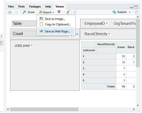
The pivot table can also be exported to an HTML file, which allows one to open it as an interactive web browser, and even better, you can send the HTML file to colleagues, which allows them to use the pivot table without having access to or changing the source data. In the Viewer window of RStudio, select the Export drop-down menu, followed by Save as Web Page…. You may be prompted to downloaded additional required packages; please click “Yes” to download these packages if you would like to save the pivot table as an HTML file. Once you have done that, you can proceed to save the file in your working directory or elsewhere. When you open (e.g., double-click on) the HTML file in the folder in which you saved it, a web browser will open with your interactive pivot table.
You can also preemptively specify the row variable(s), column variable(s), and descriptive statistic in the rpivotTable function itself. This allows you to keep a record of the different “pivots” you have applied and avoid having to drag-and-drop and point-and-click in the interactive interface. To add these specifications, we just add additional arguments (separated by commas) to the rpivotTable function. First, let’s type rows="JobLevel" (make sure the variable is in quotation marks) to set the JobLevel variable as a row. Second, let’s type cols="Sex" to set the Sex variable as a column.

Using the c (combine) function within the rpivotTable function, we can specify multiple row or column variables as a vector. For example, let’s build upon the previous syntax by adding RaceEthnicity as another column variable by typing cols=c("Sex", "RaceEthnicity").

Building upon the previous syntax even further, let’s add the argument rendererName="Heatmap" to specify that we want the pivot table to be rendered as a heatmap display.
# Access rpivotTable package
rpivotTable(demodata, rows="JobLevel", cols=c("Sex", "RaceEthnicity"), rendererName="Heatmap")
We can also render the pivot table as a treemap, where a treemap is type of data visualization in which hierarchical data are displayed as nested rectangles, such that the area of each rectangle correlates with its relative quantitative value. To create the treemap, let’s specify rows=c("Sex", "JobLevel") to indicate that the row variables are Sex and JobLevel. Next, specify rendererName="Treemap" to indicate that we want the pivot table to be rendered as a treemap.

Now it’s time to play around with applying a different type of descriptive (aggregate) statistic (as opposed to the default count (i.e., frequency) statistic). First, type rows="JobLevel" to specify JobLevel as the row variable. Second, type cols="Sex" to specify Sex as the column variable. Third, type rendererName="Bar Chart" to request that the pivot table be rendered as a Bar Chart. Fourth, type aggregatorName="Average" to specify that the average (mean) be computed for values (vals) on a specific variable (see next). Finally, type vals="AgeYrs_2019" to specify the variable (AgeYrs_2019) to be used for the calculation of the average.
# Create pivot table
rpivotTable(demodata, rows="JobLevel", cols="Sex", rendererName="Bar Chart",
            aggregatorName="Average", vals="AgeYrs_2019")