Chapter 46 Estimating the Association Between Two Categorical Variables Using Chi-Square ($\chi^2$) Test of Independence

In this chapter, we will learn how to estimate whether theoretically or practically relevant categorical (nominal, ordinal) variables are associated with employees’ decisions to voluntarily turn over. In doing so, we will learn how to estimate the chi-square ($\chi^2$) test of independence. In a previous chapter, we learned how to apply the $\chi^2$ test of independence to determine whether there was evidence of disparate impact.

46.1 Conceptual Overview

Link to conceptual video: https://youtu.be/hsCW85LqpiE

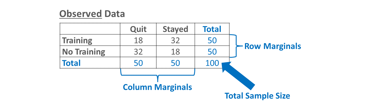
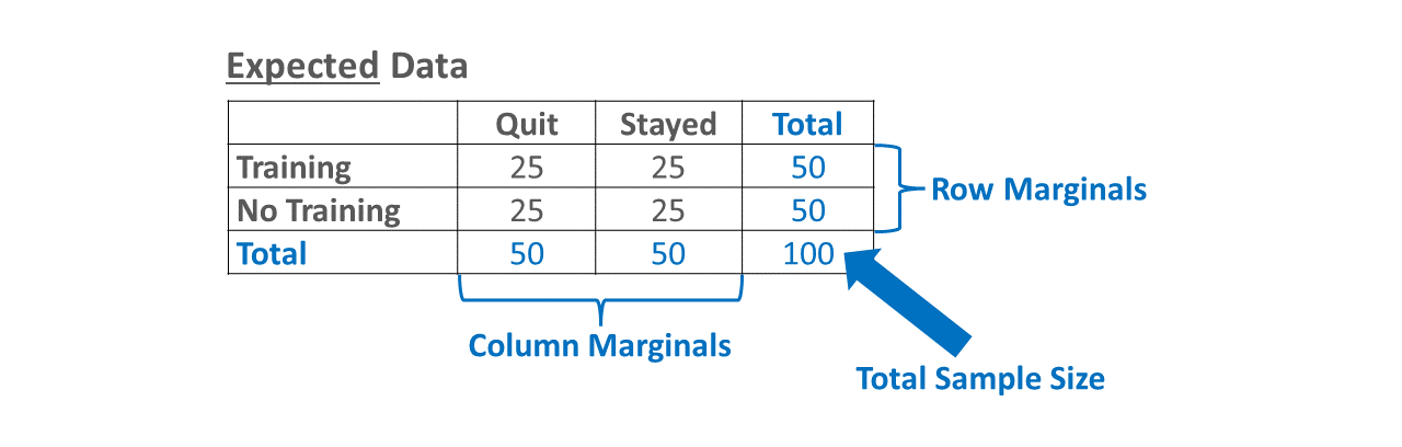
A chi-square ($\chi^2$) test of independence is a type of categorical nonparametric statistical analysis that can be used to estimate the association between two categorical (nominal, ordinal) variables. As a reminder, categorical variables do not have inherent numeric values, and thus we often just describe how many cases belong to each category (i.e., counts, frequencies). It is very common to represent the association between two categorical variables as a contingency table, which is often referred to as a cross-tabulation. A $\chi^2$ test of independence is calculated by comparing the observed data in the contingency table (i.e., what we actually found in the sample) to a model in which the variables and data in another table are distributed to be independent of one another (i.e., expected data); there are other types of expected models, but we will focus on just an independent model in this review.

The observed data includes the raw counts (i.e., frequencies) from the sample. The row and column marginals represent the sums of each row and column, respectively.

The expected data includes the counts (i.e., frequencies) that would be expected if the two categorical variables were independent of one another (i.e., not associated). The expected values for each cell are calculated by multiplying the corresponding row and column marginals and dividing that product by the total sample size.

In essence, a $\chi^2$ test of independence is used to test the null hypothesis that the two categorical variables are independent of one another (i.e., no association between them). If we reject the null hypothesis because the $\chi^2$ value relative to the degrees of freedom of the model is large enough, we conclude that the categorical variables are not in fact independent of one another but instead are contingent upon one another. In this chapter, we will focus specifically on a 2x2 $\chi^2$ test, which refers to the fact there are two categorical variables with two levels each (e.g., age: old vs. young; height: tall vs. short). As an added bonus, a 2x2 $\chi^2$ value can be converted to a phi ($\phi$) coefficient, which can be interpreted as a Pearson product-moment correlation and thus as an effect size or indicator of practical significance.

The formula for calculating $\chi^2$ is as follows:

$\chi^2 = \sum_{i = 1}^{n} \frac{(O_i - E_i)^2}{E_i}$

where $O_i$ refers to the observed values and $E_i$ refers to expected values.

The degrees of freedom ($df$) of a $\chi^2$ test is equal to the product of the number of levels of the first variable minus one and the number of levels of the second variable minus one. For example, a 2x2 $\chi^2$ test has 1 $df$: $(2-1)(2-1) = 1$

46.1.0.1 Statistical Assumptions

The statistical assumptions that should be met prior to running and/or interpreting a Pearson product-moment correlation include:

Cases are randomly sampled from the population, such that the variable scores for one individual are independent of the variable scores of another individual;
The nonoccurrences are included, where nonoccurrences refer to the instances in which an event or category does not occur. For example, when we investigate employee voluntary turnover, we often like to focus on the turnover event occurrences (i.e., quitting), but we also need to include nonoccurrences, which would be examples of the turnover event not occurring (i.e., staying). Failure to do so, could lead to misleading results.

46.1.0.2 Statistical Significance

Using null hypothesis significance testing (NHST), we interpret a p-value that is less than .05 (or whatever two- or one-tailed alpha level we set) to meet the standard for statistical significance, meaning we reject the null hypothesis that the variables are independent. If the p-value associated with $\chi^2$ value is equal to or greater than .05 (or whatever two- or one-tailed alpha level we set), then we fail to reject the null hypothesis that the categorical variables are independent. Put differently, if the p-value associated with a $\chi^2$ value is equal to or greater than .05, we conclude that there is no association between the predictor variable and the outcome variable in the population.

If we were to calculate the test by hand, then we might compare our calculated $\chi^2$ value to a table of critical values for a $\chi^2$ distribution. If our calculated value were larger than the critical value given the number of degrees of freedom (df) and the desired alpha level (i.e., significance level cutoff for p-value), we would conclude that there is evidence of an association between the categorical variables. Here is a website that lists critical values. Alternatively, we can calculate the exact p-value using statistical software if we know the exact $\chi^2$ value and the df, and most software programs compute the exact p-value automatically when estimating the $\chi^2$ test of independence.

46.1.0.3 Practical Significance

By itself, the $\chi^2$ value is not an effect size; however, in the special case of a 2x2 $\chi^2$ test of independence, we can compute a phi ($\phi$) coefficient, which can be interpreted as a Pearson product-moment correlation and thus as an effect size or indicator of practical significance. The size of a $\phi$ coefficient can be described using qualitative labels, such as small, medium, and large. The quantitative values tied to such qualitative labels of magnitude should really be treated as context specific; with that said, there are some very general rules we can apply when interpreting the magnitude of correlation coefficients, which are presented in the table below (Cohen 1992). Please note that the $\phi$ values in the table are absolute values, which means, for example, that correlation coefficients of .50 and -.50 would both have the same absolute value and thus would both be considered large.

$\phi$	Description
.10	Small
.30	Medium
.50	Large

Note: Typically, we only interpret the practical significance of an effect if the effect was found to be statistically significant. The logic is that if an effect (e.g., association, difference) is not statistically significant, then we should treat it as no different than zero, and thus it wouldn’t make sense to the interpret the size of something that statistically has no effect.

46.1.0.4 Sample Write-Up

Our organization created a new onboarding program a year ago. Today (a year later), we wish to investigate whether participating in the new vs. old onboarding program is associated with employees decisions to quit the organization for the subsequent six months. Based on a sample of 100 newcomers (N = 100) – half of whom went through the new onboarding program and half of whom went through the old onboarding program – we estimated a 2x2 chi-square ($\chi^2$) test of independence. The $\chi^2$ test of independence was statistically significant ($\chi^2$ = 7.84, df = 1, p = .04), such that those who participated in the new onboarding program were less likely to quit in their first year.

Note: If the p-value were equal to or greater than our alpha level (e.g., .05, two-tailed), then we would typically state that the association between the two variables is not statistically significant, and we would not proceed forward with interpreting the effect size (i.e., level of practical significance) because the test of statistical significance indicates that it is very unlikely based on our sample that a true association between these two variables exists in the population.

46.2 Tutorial

This chapter’s tutorial demonstrates how a chi-square test of independence can be used to identify whether an association exists between a categorical (nominal, ordinal) variable and dichotomous turnover decisions (i.e., stay vs. quit).

46.2.1 Video Tutorial

As usual, you have the choice to follow along with the written tutorial in this chapter or to watch the video tutorial below.

Link to video tutorial: https://youtu.be/l8v3kx6zNuQ

46.2.2 Functions & Packages Introduced

Function	Package
`xtabs`	base R
`print`	base R
`xtabs`	base R
`chisq.test`	base R
`prop.table`	base R
`phi`	`psych`

46.2.3 Initial Steps

If you haven’t already, save the file called “ChiSquareTurnover.csv” into a folder that you will subsequently set as your working directory. Your working directory will likely be different than the one shown below (i.e., "H:/RWorkshop"). As a reminder, you can access all of the data files referenced in this book by downloading them as a compressed (zipped) folder from the my GitHub site: https://github.com/davidcaughlin/R-Tutorial-Data-Files; once you’ve followed the link to GitHub, just click “Code” (or “Download”) followed by “Download ZIP”, which will download all of the data files referenced in this book. For the sake of parsimony, I recommend downloading all of the data files into the same folder on your computer, which will allow you to set that same folder as your working directory for each of the chapters in this book.

Next, using the setwd function, set your working directory to the folder in which you saved the data file for this chapter. Alternatively, you can manually set your working directory folder in your drop-down menus by going to Session > Set Working Directory > Choose Directory…. Be sure to create a new R script file (.R) or update an existing R script file so that you can save your script and annotations. If you need refreshers on how to set your working directory and how to create and save an R script, please refer to Setting a Working Directory and Creating & Saving an R Script.

# Set your working directory
setwd("H:/RWorkshop")

Next, read in the .csv data file called “ChiSquareTurnover.csv” using your choice of read function. In this example, I use the read_csv function from the readr package (Wickham, Hester, and Bryan 2024). If you choose to use the read_csv function, be sure that you have installed and accessed the readr package using the install.packages and library functions. Note: You don’t need to install a package every time you wish to access it; in general, I would recommend updating a package installation once ever 1-3 months. For refreshers on installing packages and reading data into R, please refer to Packages and Reading Data into R.

# Install readr package if you haven't already
# [Note: You don't need to install a package every 
# time you wish to access it]
install.packages("readr")

# Access readr package
library(readr)

# Read data and name data frame (tibble) object
cst <- read_csv("ChiSquareTurnover.csv")

## Rows: 75 Columns: 3
## ── Column specification ────────────────────────────────────────────────────────────────────────────────────────────────────────
## Delimiter: ","
## chr (3): EmployeeID, Onboarding, Turnover
## 
## ℹ Use `spec()` to retrieve the full column specification for this data.
## ℹ Specify the column types or set `show_col_types = FALSE` to quiet this message.

# Print the names of the variables in the data frame (tibble) object
names(cst)

## [1] "EmployeeID" "Onboarding" "Turnover"

# Print number of rows in data frame (tibble) object
nrow(cst)

## [1] 75

# Print structure of data frame (tibble) object
str(cst)

## spc_tbl_ [75 × 3] (S3: spec_tbl_df/tbl_df/tbl/data.frame)
##  $ EmployeeID: chr [1:75] "E1" "E2" "E3" "E8" ...
##  $ Onboarding: chr [1:75] "No" "No" "No" "No" ...
##  $ Turnover  : chr [1:75] "Quit" "Quit" "Quit" "Quit" ...
##  - attr(*, "spec")=
##   .. cols(
##   ..   EmployeeID = col_character(),
##   ..   Onboarding = col_character(),
##   ..   Turnover = col_character()
##   .. )
##  - attr(*, "problems")=<externalptr>

# Print first 6 rows of data frame (tibble) object
head(cst)

## # A tibble: 6 × 3
##   EmployeeID Onboarding Turnover
##   <chr>      <chr>      <chr>   
## 1 E1         No         Quit    
## 2 E2         No         Quit    
## 3 E3         No         Quit    
## 4 E8         No         Quit    
## 5 E14        No         Quit    
## 6 E22        No         Quit

There are 3 variables and 75 cases (i.e., employees) in the cst data frame: EmployeeID, Onboarding, and Turnover. Per the output of the str (structure) function above, all of the variables are of type character. EmployeeID is the unique employee identifier variable. Onboarding is a variable that indicates whether new employees participated in the onboarding program, and it has two levels: did not participate (No) and did participate (Yes) Turnover is a variable that indicates whether these individuals left the organization during their first year; it also has two levels: Quit and Stayed.

46.2.4 Create a Contingency Table for Observed Data

Before running the chi-square test, we need to create a contingency (cross-tabulation) table for the Onboarding and Turnover variables. To do so, we will use the xtabs function from base R. In the function parentheses, as the first argument type the ~ operator followed by the two variables names, separated by the + operator (i.e., ~ Onboarding + Turnover). As the second argument, type data= followed by the name of the data frame to which both variables belong (cst). We will use the <- assignment operator to name the table object (tbl). For more information on creating tables, check out the chapter on summarizing two or more categorical variables using cross-tabulations.

# Create two-way contingency table
tbl <- xtabs(~ Onboarding + Turnover, data=cst)

Let’s print the new tbl object to your Console.

# Print table
print(tbl)

##           Turnover
## Onboarding Quit Stayed
##        No    16      7
##        Yes    6     46

As you can see, we have created a 2x2 contingency table, as it has two variables (Onboarding, Turnover) with each variable consisting of two levels (i.e., categories). This table includes our observed data.

46.2.5 Estimate Chi-Square ($\chi^2$) Test of Independence

Using the contingency table we created called tbl, we will insert it as the sole parenthetical argument in the chisq.test function from base R.

# Estimate chi-square test of independence
chisq.test(tbl)

## 
##  Pearson's Chi-squared test with Yates' continuity correction
## 
## data:  tbl
## X-squared = 23.179, df = 1, p-value = 0.000001476

In the output, note that the $\chi^2$ value is 23.179 with 1 degree of freedom (df), and the associated p-value is less than .05, leading us to reject the null hypothesis that these two variables are independent of one another ($\chi^2$ = 23.176, df = 1, p < .001). In other words, we have concluded that there is a statistically significant association between onboarding participation and whether someone quits in the first year.

To understand the nature of this association, we need to look back to the contingency table values. In fact, sometimes it is helpful to look at the column (or row) proportions by applying the prop.table function from base R to the tbl object we created. As the second argument, type the numeral 2 to request the column marginal proportions.

# Print column marginal proportions
prop.table(tbl, 2)

##           Turnover
## Onboarding      Quit    Stayed
##        No  0.7272727 0.1320755
##        Yes 0.2727273 0.8679245

As you can see from the contingency table, of those employees who stayed, proportionally more employees had participated in the onboarding program (86.8%). Alternatively, for those who quit, proportionally more employees did not participate in the onboarding program (72.7%). Given our interpretation of the table along with the significant $\chi^2$ test, we can conclude that employees were significantly more likely to stay through the end of their first year if they participated in the onboarding program.

In the special case of a 2x2 contingency table (or a 1x4 vector), we can compute a phi ($\phi$) coefficient, which can be interpreted like a Pearson product-moment correlation coefficient and thus as an effect size. To calculate the phi coefficient, we will use the phi function from the psych package (Revelle 2023). If you haven’t already, install and access the psych package.

# Install package
install.packages("psych")

# Access package
library(psych)

Within the phi function parentheses, insert the name of the 2x2 contingency table object (tbl) as the sole argument.

# Estimate phi coefficient
phi(tbl)

## [1] 0.587685

The $\phi$ coefficient for the association between Onboarding and Turnover is .59, which by conventional correlation standards is a large effect ($\phi$ = .59). Here is a table containing conventional rules of thumb for interpreting a Pearson correlation coefficient (r) or a phi coefficient ($\phi$) as an effect size:

$\phi$	Description
.10	Small
.30	Medium
.50	Large

Technical Write-Up: Based on a sample of 75 employees, we investigated whether participating in an onboarding program was associated with new employees’ decisions to quit in the first 12 months. Using a chi-square ($\chi^2$) test of independence, we found that new employees who participated in the onboarding program were less likely to quit during their first 12 months on the job ($\chi^2$ = 23.176, df = 1, p < .001). Specifically, of those employees who stayed at the organization, proportionally more employees had participated in the onboarding program (86.8%), and of those employees who quit the organization, proportionally more employees did not participate in the onboarding program (72.7%). The magnitude of this effect can be described as large ($\phi$ = .59).

46.2.5.1 Optional: Print Observed and Expected Counts

In some instances, it might be helpful to view the observed and expected, as these are the basis for estimating the $\chi^2$ test of independence. First, we need to create an object that contains the information from the chisq.test function. Using the <- assignment operator, let’s name this object chisq.

# Create chi-square object
chisq <- chisq.test(tbl)

We can request the observed counts/frequencies by typing the name of the chisq object, followed by the $ operator and observed. These will look familiar because they are the counts from our original contingency table.

# Request observed counts/frequencies
chisq$observed

##           Turnover
## Onboarding Quit Stayed
##        No    16      7
##        Yes    6     46

To request the expected counts/frequencies, type the name of the chisq object, followed by the $ operator and expected.

# Request expected counts/frequencies
chisq$expected

##           Turnover
## Onboarding      Quit   Stayed
##        No   6.746667 16.25333
##        Yes 15.253333 36.74667

We can descriptively see departures from the observed and expected values in a systematic manner.

To understand which cells were most influential in the calculation of the $\chi^2$ value, it is straightforward to request the Pearson residuals. Pearson residuals with larger absolute values have bigger contributions to the $\chi^2$ value.

# Request Pearson residuals
chisq$residuals

##           Turnover
## Onboarding      Quit    Stayed
##        No   3.562489 -2.295234
##        Yes -2.369277  1.526473

46.2.6 Summary

In this chapter, we learned how to estimate a chi-square ($\chi^2$) test of independence using the chisq.test function from base R.

46.3 Chapter Supplement

In this chapter supplement, you will have an opportunity to learn how to compute and interpret an odds ratio and its 95% confidence interval, where the odds ratio is another method we can use to describe the association between two categorical variables from a 2x2 contingency table.

46.3.1 Functions & Packages Introduced

Function	Package
`sqrt`	base R
`exp`	base R
`log`	base R
`print`	base R

46.3.2 Initial Steps

If required, please refer to the Initial Steps section from this chapter for more information on these initial steps.

# Set your working directory
setwd("H:/RWorkshop")

# Install readr package if you haven't already
# [Note: You don't need to install a package every 
# time you wish to access it]
install.packages("readr")

# Access readr package
library(readr)

# Read data and name data frame (tibble) object
cst <- read_csv("ChiSquareTurnover.csv")

## Rows: 75 Columns: 3
## ── Column specification ────────────────────────────────────────────────────────────────────────────────────────────────────────
## Delimiter: ","
## chr (3): EmployeeID, Onboarding, Turnover
## 
## ℹ Use `spec()` to retrieve the full column specification for this data.
## ℹ Specify the column types or set `show_col_types = FALSE` to quiet this message.

# Print the names of the variables in the data frame (tibble) object
names(cst)

## [1] "EmployeeID" "Onboarding" "Turnover"

# View variable type for each variable in data frame (tibble) object
str(cst)

## spc_tbl_ [75 × 3] (S3: spec_tbl_df/tbl_df/tbl/data.frame)
##  $ EmployeeID: chr [1:75] "E1" "E2" "E3" "E8" ...
##  $ Onboarding: chr [1:75] "No" "No" "No" "No" ...
##  $ Turnover  : chr [1:75] "Quit" "Quit" "Quit" "Quit" ...
##  - attr(*, "spec")=
##   .. cols(
##   ..   EmployeeID = col_character(),
##   ..   Onboarding = col_character(),
##   ..   Turnover = col_character()
##   .. )
##  - attr(*, "problems")=<externalptr>

# View first 6 rows of data frame (tibble) object
head(cst)

## # A tibble: 6 × 3
##   EmployeeID Onboarding Turnover
##   <chr>      <chr>      <chr>   
## 1 E1         No         Quit    
## 2 E2         No         Quit    
## 3 E3         No         Quit    
## 4 E8         No         Quit    
## 5 E14        No         Quit    
## 6 E22        No         Quit

46.3.3 Compute Odds Ratio for 2x2 Contingency Table

When communicating the association between two categorical variables, sometimes it helps to the express the association as an odds ratio. An odds ratio allows us to describe the association between two variables as, “given X, the odds of experiencing the event are Y times greater.”

To get started, let’s create a 2x2 contingency table object called tbl, which will house the counts for our two categorical variables (Onboarding, Turnover), where each variable has two levels.

# Create two-way contingency table
tbl <- xtabs(~ Onboarding + Turnover, data=cst)

# Print table
print(tbl)

##           Turnover
## Onboarding Quit Stayed
##        No    16      7
##        Yes    6     46

I’m going to demonstrate how to manually compute the odds ratio for a 2x2 contingency table, but note that you can estimate a logistic regression model to arrive at the same end, which is covered in the chapter on identifying predictors of turnover. I should also note that there are some great functions out there like the oddsratio.wald function from the epitools package that will do these calculations for us; nonetheless, I think it’s worthwhile to unpack how relatively simple these calculations are, as this can serve as a nice warm up for the following chapter.

When we have a 2x2 contingency table of counts, the odds ratio is relatively straightforward to calculate if we conceptualize our contingency table as follows. Because we are expecting that those who participate in the treatment (i.e., onboarding program) will be more likely to stay in the organization, let’s frame the act of staying as the focal event, which means that those who quit did not experience the event of staying.

Condition	No Event (Quit)	Event (Stayed)
Control (No Onboarding)	D	C
Treatment (Onboarding)	B	A

The formula for computing an odds ratio is:

$OR = \frac{\frac{A}{C}}{\frac{B}{D}}$

where:

A is the number of individuals who participated in the treatment condition (e.g., onboarding program) and who also experienced the event in question (e.g., stayed);
B is the number of individuals who participated in the treatment condition (e.g., onboarding program) but who did not experience the event in question (e.g., quit);
C is the number of individuals who participated in the control condition (e.g., no onboarding program) but who also experienced the event in question (e.g., stayed);
D is the number of individuals who participated in the control condition (e.g., no onboarding program) and who did not experience the event in question (e.g., quit).

The formula can also be written in the following manner after cross-multiplication, which is what we’ll use when computing the odds ratio, as I think it is easier to read in R:

$OR = \frac{A \times D}{B \times C}$

To make our calculations clearer, let’s reference specific cells from our contingency table object (tbl) using brackets ([ ]), where the first value within brackets references the row number and the second references the column number. We’ll assign the count value from each score to objects A, B, C, and D, to be consistent with the above formula.

# Assign counts to objects
A <- tbl[2,2]
B <- tbl[2,1]
C <- tbl[1,2]
D <- tbl[1,1]

Next, we will plug objects A, B, C, and D into the formula (see above) using the multiplication (*) and division (/) operators, and assign the result to an object called OR using the <- assignment operator.

# Calculate odds ratio of someone *staying* 
# who participated in the treatment (onboarding program)
OR <- (A * D) / (B * C)

# Print odds ratio
print(OR)

## [1] 17.52381

The odds ratio is 17.52, which indicates that for those who participated in the onboarding program the odds of staying was 17.52 greater. If an odds ratio is equal to 1.00, then it signifies no association – or equal odds of experiencing the focal event. If an odds ratio is greater than 1.00, then it signifies a positive association between the two variables, such that the higher level on the first variable (e.g., receiving treatment) is associated with the higher level on the second variable (e.g., experiencing event).

Alternatively, if we would like to, instead, understand the odds of someone quitting after participating in the onboarding program, we would flip the numerator and denominator from our above code. Effectively, in this example, this simple operation switches our focal event from staying to quitting, thereby giving us a different perspective on the association between the two variables.

# Calculate odds ratio of someone *quitting* 
# who participated in the treatment (onboarding program)
OR_alt <- (B * C) / (A * D) # flip numerator and denominator 

# Print odds ratio
print(OR_alt)

## [1] 0.05706522

The new odds ratio (OR_alt) is approximately .06 (with rounding). Because an odds ratio that is less than 1.00 signifies a negative association, this odds ratio indicates that those who participated in the treatment (onboarding program) are less likely to have experienced the event of quitting. If we compute the reciprocal of the odds ratio, we arrive back at our original odds ratio.

# Calculate reciprocal of odds ratio
1 / OR_alt

## [1] 17.52381

This takes us back to our original interpretation, which is that for those who participated in the onboarding program the odds of staying was 17.52 greater. I should note that an odds ratio of 17.52 is a HUGE effect.

When working with a 2x2 contingency table, I recommend computing the reciprocal of any odds ratio less than 1.00, as it often leads to a more straightforward interpretation – just remember that the we have to conceptually flip the event and non-event when interpreting the now positive association between the two categorical variables.

As a significance test for the odds ratio, we can compute the 95% confidence intervals. Because an odds ratio of 1.00 signifies no association between the two variables, any confidence interval that does not include 1.00 will be considered statistically significant.

To compute the confidence interval, we first need to compute the standard error of the odds ratio using the following formula.

$SE = \sqrt{\frac{1}{A} + \frac{1}{B} + \frac{1}{C} + \frac{1}{D}}$

# Calculate standard error (SE) of odds ratio
SE <- sqrt((1/A) + (1/B) + (1/C) + (1/D))

To construct the lower and upper limits of a 95% confidence interval, we need to first multiply the standard error (SE) by 1.96. To compute the lower limit, we subtract that product from the natural log of odds ratio (log(OR)) and then exponentiate the resulting value using the exp function from base R, where the exp function takes Euler’s constant ($e$) and adds a specified exponent to it. To compute the upper limit, we add that product to the natural log of odds ratio and then exponentiate the resulting value.

# Calculate 95% confidence interval for odds ratio
exp(log(OR) - 1.96*SE) # lower limit

## [1] 5.122538

exp(log(OR) + 1.96*SE) # upper limit

## [1] 59.94761

The 95% confidence interval ranges from 5.12 to 59.95 (95% CI[5.12, 59.95]). Because this interval does not include 1.00, we can conclude that the odds ratio of 17.52 is statistically significantly different from 1.00.

References

Cohen, Jacob. 1992. “A Power Primer.” Psychological Bulletin 112 (1): 155–59.

Revelle, William. 2023. Psych: Procedures for Psychological, Psychometric, and Personality Research. https://personality-project.org/r/psych/

Wickham, Hadley, Jim Hester, and Jennifer Bryan. 2024. Readr: Read Rectangular Text Data. https://CRAN.R-project.org/package=readr.

R for HR:
An Introduction to Human Resource Analytics Using R

Chapter 46 Estimating the Association Between Two Categorical Variables Using Chi-Square (\(\chi^2\)) Test of Independence