Chapter 20 Manipulating & Restructuring Data
In this chapter, we will learn how to manipulate and restructure data – and more specifically, convert a data frame object from wide to long format and from long to wide format.
20.1 Conceptual Overview
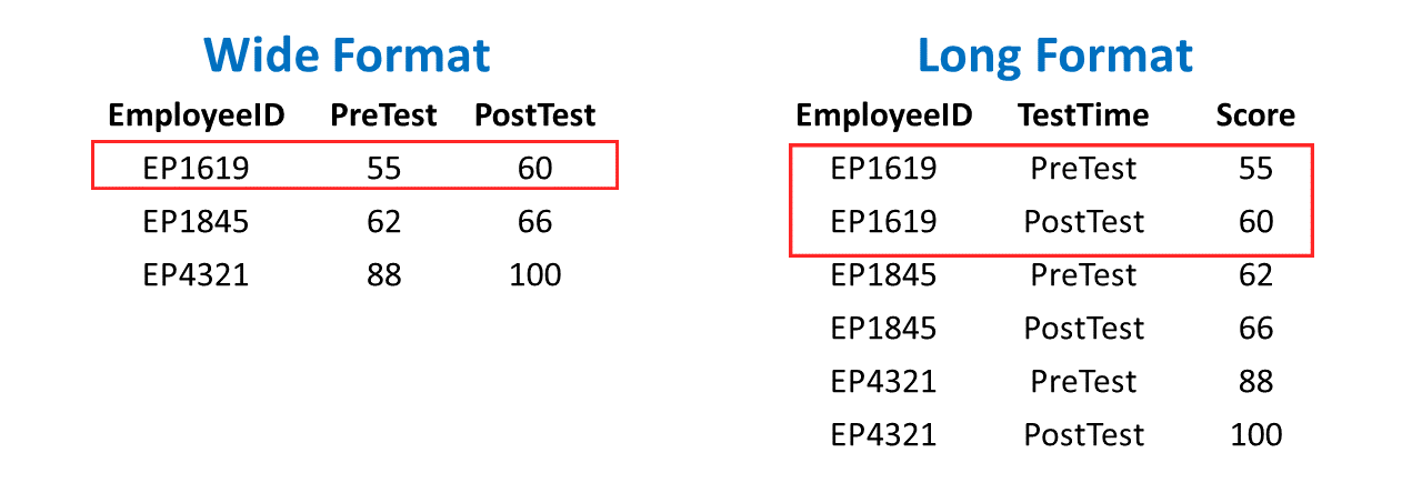
Data manipulation and restructuring refers to the process in which data are restructured or formatted in a different manner. When we think about structured data, we often think in terms of wide versus long formats. Wide format data are structured such that there are more columns (i.e., variables) and fewer rows than with long format data. For example, most survey platforms allow you to download the survey responses in a wide format, such that each variable (that corresponds to a survey item/question) will have its own column. Long format data are structured such that that are (sometimes) fewer columns yet more rows than with wide-format data. For example, we can restructure survey data from wide format such that one variable (i.e., column) contains the names of the different survey items/questions, and another variable contains the responses/scores for each item/question. Often our decision to manipulate data into wide versus long formats has to do with the type of analysis or visualization we plan to perform. As such, understanding how to manipulate and restructure your data is an important data-science skill.
20.2 Tutorial
This chapter’s tutorial demonstrates how to restructure data from wide to long format and from long to wide format.
20.2.1 Video Tutorial
In the video tutorial below, I demonstrate how to use two data-manipulation functions that have since been deprecated by the tidyr package, which are called gather and spread. In this chapter, I review how to use the new data-manipulation functions from the tidyr package called pivot_longer and pivot_wider, respectively. I personally find the new functions to be more intuitive to use, but perhaps you’ll disagree. Regardless of which you choose, both will help you manipulate data from wide to long format and from long to wide format.
Link to video tutorial: https://youtu.be/5DgEAKLRjhw
20.2.2 Functions & Packages Introduced
| Function | Package |
|---|---|
pivot_longer |
tidyr |
c |
base R |
pivot_wider |
tidyr |
20.2.3 Initial Steps
If you haven’t already, save the file called “ManipulatingData.csv” into a folder that you will subsequently set as your working directory. Your working directory will likely be different than the one shown below (i.e., "H:/RWorkshop"). As a reminder, you can access all of the data files referenced in this book by downloading them as a compressed (zipped) folder from the my GitHub site: https://github.com/davidcaughlin/R-Tutorial-Data-Files; once you’ve followed the link to GitHub, just click “Code” (or “Download”) followed by “Download ZIP”, which will download all of the data files referenced in this book. For the sake of parsimony, I recommend downloading all of the data files into the same folder on your computer, which will allow you to set that same folder as your working directory for each of the chapters in this book.
Next, using the setwd function, set your working directory to the folder in which you saved the data file for this chapter. Alternatively, you can manually set your working directory folder in your drop-down menus by going to Session > Set Working Directory > Choose Directory…. Be sure to create a new R script file (.R) or update an existing R script file so that you can save your script and annotations. If you need refreshers on how to set your working directory and how to create and save an R script, please refer to Setting a Working Directory and Creating & Saving an R Script.
Next, read in the .csv data file called “ManipulatingData.csv” using your choice of read function. In this example, I use the read_csv function from the readr package (Wickham, Hester, and Bryan 2024). If you choose to use the read_csv function, be sure that you have installed and accessed the readr package using the install.packages and library functions. Note: You don’t need to install a package every time you wish to access it; in general, I would recommend updating a package installation once ever 1-3 months. For refreshers on installing packages and reading data into R, please refer to Packages and Reading Data into R.
# Install readr package if you haven't already
# [Note: You don't need to install a package every
# time you wish to access it]
install.packages("readr")
# Access readr package
library(readr)
# Read data and name data frame (tibble) object
datam <- read_csv("ManipulatingData.csv")## Rows: 20 Columns: 5
## ── Column specification ────────────────────────────────────────────────────────────────────────────────────────────────────────────
## Delimiter: ","
## dbl (5): SurveyID, JobSatisfaction, TurnoverIntentions, OrgCommitment, JobInvolvement
##
## ℹ Use `spec()` to retrieve the full column specification for this data.
## ℹ Specify the column types or set `show_col_types = FALSE` to quiet this message.## [1] "SurveyID" "JobSatisfaction" "TurnoverIntentions" "OrgCommitment" "JobInvolvement"## # A tibble: 20 × 5
## SurveyID JobSatisfaction TurnoverIntentions OrgCommitment JobInvolvement
## <dbl> <dbl> <dbl> <dbl> <dbl>
## 1 1 55.4 97.2 32.3 50.5
## 2 2 51.5 96 53.4 50.3
## 3 3 46.2 94.5 63.9 50.2
## 4 4 42.8 91.4 70.3 50.3
## 5 5 40.8 88.3 34.1 50.5
## 6 6 38.7 84.9 67.7 30.5
## 7 7 35.6 79.9 53.3 30.5
## 8 8 33.1 77.6 63.5 30.5
## 9 9 29 74.5 68 30.5
## 10 10 26.2 71.4 67.4 30.5
## 11 11 23.1 66.4 15.6 30.5
## 12 12 22.3 61.8 71.8 30.5
## 13 13 22.3 57.2 70.2 30.6
## 14 14 23.3 52.9 64.9 30.5
## 15 15 25.9 51 62.2 30.5
## 16 16 29.5 51 67.3 30.5
## 17 17 32.8 51 40.6 30.5
## 18 18 35.4 51.4 74.7 30.5
## 19 19 40.3 51.4 71.8 50.1
## 20 20 56.7 56 84.3 69.5Note in the data frame that the SurveyID variable (i.e., column, field) is a unique identifier variable, which means that each case (i.e., observation) has a unique value on this variable. Each row represents a unique employee’s composite score on four measures (i.e., JobSatisfaction, TurnoverIntentions, OrgCommitment, JobInvolvement), where higher scores indicate higher levels of the concept (i.e., construct) being measured.
## [1] 20Note how the data frame currently has 20 rows (cases) of data, as shown by the output to the nrow function from base R.
20.2.4 Wide-to-Long Format Data Manipulation
The data frame we read in called datam is in wide format, as each substantive variable has its own column. To restructure the data from wide to long format, we will use the pivot_longer function from the tidyr package (Wickham, Vaughan, and Girlich 2023). Along with readr and dplyr (as well as other useful packages), the tidyr package is part of the tidyverse of packages. Let’s begin by installing and accessing the tidyr package so that we can use the pivot_longer function.
If you received an error when attempting to access the tidyr package using the library function, you may need to install the following packages using the install.packages function: rlang and glue. Alternatively, you may try installing the entire tidyverse package.
Now that we’ve accessed the tidyr package, I will demonstrate two techniques for applying the pivot_longer function.
The first technique uses the pipe operator (%>%). The pipe operator comes from a package called magrittr (Bache and Wickham 2022), on which the tidyr package is partially dependent. In short, a pipe allows a person to more efficiently write code and to improve the readability of the code and overall script. Specifically, a pipe forwards the result or value of one object or expression to a subsequent function. In doing so, one can avoid writing functions in which other functions are nested parenthetically. For more information on the pipe operator, check out Wickham and Grolemund’s (2017) chapter on pipes.
The second technique for applying the pivot_longer function takes a more traditional approach in that it involves nested functions being nested parenthetically. If you don’t want to learn how to use pipes (or would like to learn how to use them at a later date), feel free to skip to the section below called Without Pipe.
20.2.4.1 With Pipe
Using the pipe (%>%) operator technique, let’s apply the pivot_longer function to manipulate the datam data frame object from wide format to long format.
We can specify the wide-to-long manipulation as follows.
- Create a name for a new data frame object to which we will eventually assign a long-format data frame object; here, I name the new data frame object
datam_long. - Use the
<-operator to assign the new long-form data frame object to the object nameddatam_longin the step above. - Type the name of the original data frame object (
datam), followed by the pipe (%>%) operator. - Type the name of the
pivot_longerfunction.
- As the first argument in the
pivot_longerfunction, typecols=followed by thec(combine) function. As the arguments within thecfunction, list the names of the variables that you wish to pivot from separate variables (wide) to levels or categories of a new variable, effectively stacking them vertically. In this example, let’s list the names of the four survey measures:JobSatisfaction,TurnoverIntentions,OrgCommitment, andJobInvolvement. - As the second argument in the
pivot_longerfunction, typenames_to=followed by what you would like to name the new stacked variable (see previous) created from the four survey measure variables. Let’s call the new variable containing the names of the measures the following:"Measure". - As the third argument in the
pivot_longerfunction, typevalues_to=followed by what you would like to name the new variable that contains the scores for the four survey variables that are now stacked vertically for each case. Let’s call the new variable containing the scores on the four measures the following:"Score".
# Apply pivot_longer function to restructure data in long format (using pipe)
datam_long <- datam %>%
  pivot_longer(cols=c(JobSatisfaction, TurnoverIntentions, OrgCommitment, JobInvolvement),
               names_to="Measure",
               values_to="Score")

# Print first 12 rows of new data frame
head(datam_long, n=12)
## # A tibble: 12 × 3
## SurveyID Measure Score
## <dbl> <chr> <dbl>
## 1 1 JobSatisfaction 55.4
## 2 1 TurnoverIntentions 97.2
## 3 1 OrgCommitment 32.3
## 4 1 JobInvolvement 50.5
## 5 2 JobSatisfaction 51.5
## 6 2 TurnoverIntentions 96
## 7 2 OrgCommitment 53.4
## 8 2 JobInvolvement 50.3
## 9 3 JobSatisfaction 46.2
## 10 3 TurnoverIntentions 94.5
## 11 3 OrgCommitment 63.9
## 12 3 JobInvolvement 50.2As you can see, in the output, each respondent now has four rows of data – one row for each measure and the associated score. The giveaway is that each respondent’s unique SurveyID value is repeated four times.
## [1] "SurveyID" "Measure" "Score"Note how there are now just three variables: SurveyID, Measure, and Score. Further, by applying the nrow function to the new data frame (as shown below), we can see that the new data frame is now much longer in terms of the number of rows; specifically, the original datam data frame in wide format has 20 rows, and now the new datam_long data frame in long format has 80 rows.
## [1] 80Now apply the View function from base R to view and scroll through the whole data frame. Note that the unique identifier variable (i.e., SurveyID) repeats multiple times to indicate that the same survey respondent has scores in multiple rows.
20.2.4.2 Without Pipe
We can also apply the pivot_longer function without using the pipe (%>%) operator. To do so, use the same code as above, except drop the pipe (%>%) operator and type data= followed by the name of the original data frame (datam) as the first argument within the pivot_longer function parentheses.
# Apply pivot_longer function to restructure data in long format (without using pipe)
datam_long <- pivot_longer(data=datam,
                           cols=c(JobSatisfaction, TurnoverIntentions, OrgCommitment, JobInvolvement),
                           names_to="Measure",
                           values_to="Score")

# Print first 12 rows of new data frame
head(datam_long, n=12)
## # A tibble: 12 × 3
## SurveyID Measure Score
## <dbl> <chr> <dbl>
## 1 1 JobSatisfaction 55.4
## 2 1 TurnoverIntentions 97.2
## 3 1 OrgCommitment 32.3
## 4 1 JobInvolvement 50.5
## 5 2 JobSatisfaction 51.5
## 6 2 TurnoverIntentions 96
## 7 2 OrgCommitment 53.4
## 8 2 JobInvolvement 50.3
## 9 3 JobSatisfaction 46.2
## 10 3 TurnoverIntentions 94.5
## 11 3 OrgCommitment 63.9
## 12 3 JobInvolvement 50.2Regardless of whether we use the pipe (%>%) operator, we end up with the same wide-to-long format manipulation.
20.2.5 Long-to-Wide Format Data Manipulation
Using the long-format data frame we just created called datam_long, let’s manipulate it back to wide format using the pivot_wider function from the tidyr package. As we did above, we’ll do the long-to-wide data manipulation with and without the pipe (%>%) operator.
20.2.5.1 With Pipe
Using the pipe (%>%) operator technique, let’s apply the pivot_wider function to manipulate the datam_long data frame object from long format back to wide format.
We can specify the long-to-wide manipulation as follows.
- Create a name for a new data frame object to which we will eventually assign a long-format data frame object; here, I name the new data frame object
datam_wide. - Use the
<-operator to assign the new wide-form data frame object to the object nameddatam_widein the step above. - Type the name of the long-format data frame object (
datam_long), followed by the pipe (%>%) operator. - Type the name of the
pivot_widerfunction.
- As the first argument in the
pivot_widerfunction, typenames_from=followed by the name of the variable that contains the names of the different survey measures:Measure. The levels or categories of thisMeasurevariable will become the names of separate columns (i.e., variables) when the long-format data frame object is converted to a wide-format data frame object. - As the second argument in the
pivot_widerfunction, typevalues_from=followed by the name of the variable that contains the values (i.e., scores) for each of the survey measures:Score. The values from theScorevariable will provide the data for the new survey-measure variables when the data frame object is in wide format.
# Apply pivot_wider function to restructure data in wide format (using pipe)
datam_wide <- datam_long %>%
  pivot_wider(names_from=Measure,
              values_from=Score)

# Print first 12 rows of new data frame
head(datam_wide, n=12)
## # A tibble: 12 × 5
## SurveyID JobSatisfaction TurnoverIntentions OrgCommitment JobInvolvement
## <dbl> <dbl> <dbl> <dbl> <dbl>
## 1 1 55.4 97.2 32.3 50.5
## 2 2 51.5 96 53.4 50.3
## 3 3 46.2 94.5 63.9 50.2
## 4 4 42.8 91.4 70.3 50.3
## 5 5 40.8 88.3 34.1 50.5
## 6 6 38.7 84.9 67.7 30.5
## 7 7 35.6 79.9 53.3 30.5
## 8 8 33.1 77.6 63.5 30.5
## 9 9 29 74.5 68 30.5
## 10 10 26.2 71.4 67.4 30.5
## 11 11 23.1 66.4 15.6 30.5
## 12 12 22.3 61.8 71.8 30.5Now let’s print the variable names in the new datam_wide data frame object.
## [1] "SurveyID" "JobSatisfaction" "TurnoverIntentions" "OrgCommitment" "JobInvolvement"Note how we are now back to the same variables from our original wide-format data frame called datam: SurveyID, JobInvolvement, JobSatisfaction, OrgCommitment, and TurnoverIntentions. Further, by applying the nrow function to the new data frame (as shown below), we can see that the new wide-format data frame is now back to 20 rows. We have come full circle, as the pivot_wider function complements the pivot_longer function.
## [1] 2020.2.5.2 Without Pipe
We can also apply the pivot_wider function without the pipe (%>%) operator. Simply use the same code as above, except drop the pipe (%>%) operator and type data= followed by the name of the long-format data frame object (datam_long) as the first argument within the pivot_wider function parentheses.
# Apply pivot_wider function to restructure data in wide format (without using pipe)
datam_wide <- pivot_wider(data=datam_long,
                          names_from=Measure,
                          values_from=Score)

# Print first 12 rows of new data frame
head(datam_wide, n=12)
## # A tibble: 12 × 5
## SurveyID JobSatisfaction TurnoverIntentions OrgCommitment JobInvolvement
## <dbl> <dbl> <dbl> <dbl> <dbl>
## 1 1 55.4 97.2 32.3 50.5
## 2 2 51.5 96 53.4 50.3
## 3 3 46.2 94.5 63.9 50.2
## 4 4 42.8 91.4 70.3 50.3
## 5 5 40.8 88.3 34.1 50.5
## 6 6 38.7 84.9 67.7 30.5
## 7 7 35.6 79.9 53.3 30.5
## 8 8 33.1 77.6 63.5 30.5
## 9 9 29 74.5 68 30.5
## 10 10 26.2 71.4 67.4 30.5
## 11 11 23.1 66.4 15.6 30.5
## 12 12 22.3 61.8 71.8 30.5Regardless of whether we use the pipe (%>%) operator, we end up with the same long-to-wide format manipulation.
20.2.6 Summary
In this chapter, we learned how to manipulate a data frame from wide format to long format using the pivot_longer, and how to manipulate a data frame from long format to wide format using the pivot_wider. Both functions are from the tidyr package. Manipulating and restructuring data into different formats or structures is often an essential data-management step prior to running certain analyses or generating certain data visualizations.