Chapter 56 Estimating a Mediation Model Using Path Analysis
In this chapter, we will learn how to estimate a mediation analysis using path analysis.
56.1 Conceptual Overview
Mediation analysis is used to investigate whether an intervening variable transmits the effects of a predictor variable on an outcome variable. Both multiple regression and structural equation modeling (path analysis) can be used to perform mediation analysis, but structural equation modeling (path analysis) offers a single-step process that often more efficient. When implemented using path analysis, mediation analysis follows the same model specification, model identification, and model fit considerations as general applications of path analysis. For more information on path analysis, please refer to the previous chapter on path analysis.
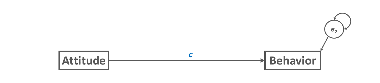
Just as in a conventional path analysis model, we often represent our mediation analysis model visually as a path diagram. For illustration purposes, let’s begin with a path diagram of the direct relation between a predictor variable called Attitude with an outcome variable called Behavior (see Figure 1). This path diagram specifies Attitude (towards the Behavior) as a predictor of the Behavior, with any error in prediction captured in the (residual) error term. By convention, we commonly refer to this path as the c path.
In the path diagram depicted in Figure 2, we introduce an intervening variable, which we commonly refer to as the mediator variable – or just as the mediator. As we saw in Figure 1, a direct relation between the predictor variable Attitude and the outcome variable Behavior is shown; however, note that we now refer to this relation as the c’ path (spoken: “c prime”) because it represents the direct effect of the predictor variable on the outcome variable in the presence of (i.e., statistically controlling) for the effect of the mediator variable. The mediator variable is called Intention, and as you can see, it intervenes between the predictor and outcome variables. The direct relation between the predictor variable and mediator variable is commonly referred to as the a path, and note that because the mediator variable is an endogenous variable (i.e., has a specified cause in the model), it as a (residual) error term. The direct relation between the mediator variable and the outcome variable is commonly referred to as the b path. The effect of the predictor variable on the outcome variable via the mediating variable is referred to as the indirect effect given that the predictor variable indirectly influences the outcome variable through another variable; in other words, the mediator variable transmits the effect of the predictor variable to the outcome variable.
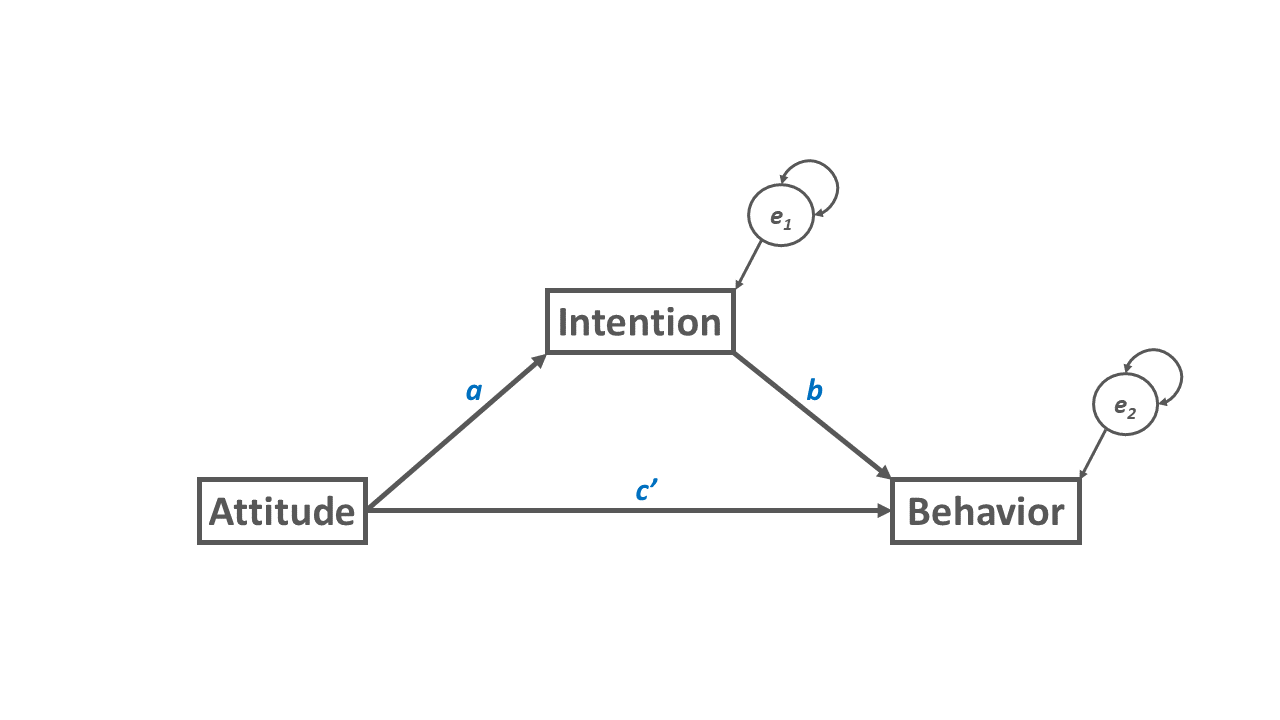
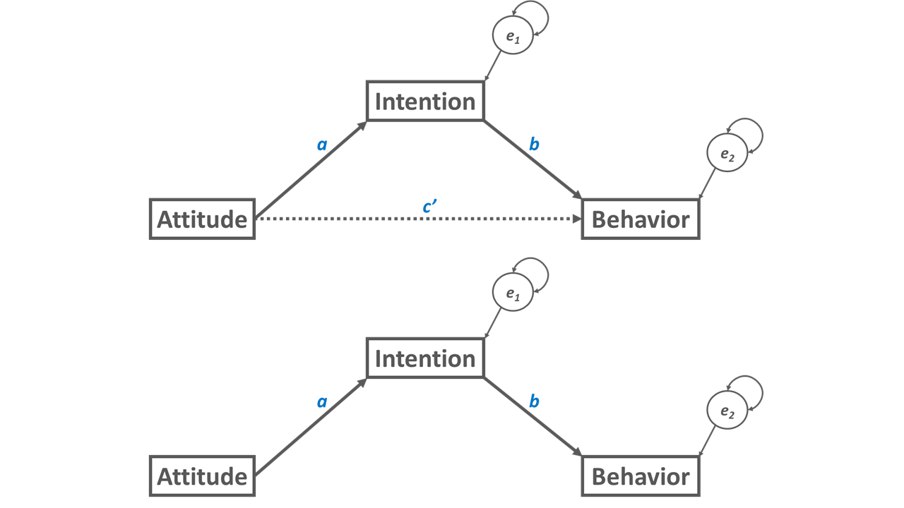
The mediation model shown in Figure 2 is an example of a partial mediation. We can distinguish between a partial and a complete mediation. A partial mediation is a mediation in which the direct relation (c’) between the predictor variable and the outcome variable is non-zero; in other words, a direct relation between the predictor and the outcome is estimated as a free parameter. A complete mediation (i.e., full mediation) is a mediation in which the direct relation (c’) between the predictor variable and the outcome variable is zero; in other words, the direct relation between the predictor and the outcome is fixed at zero, which means we don’t specify the direct relation at all in our model – or we specify the direct relation but fix it to zero. A complete mediation is shown in Figure 3.
56.1.1 Estimation of Indirect Effect
There are different approaches to estimating the indirect effect, such as causal steps (Baron and Kenny 1986), difference in coefficients, and product of coefficients (MacKinnon and Dwyer 1993). Because the product of coefficients approach is efficient to implement, we will focus on that approach in this tutorial. Using this approach, the indirect effect is estimated by computing the product of the coefficients for directional relations (i.e., paths), which include the relation between the predictor variable and the mediator variable (a path) and the relation between the mediator variable and the outcome variable (b). The statistical significance of the indirect effect can be computed by dividing the product of the coefficients by its standard error, and then the resulting ratio (quotient) can be compared to a standard normal distribution – or another distribution.
There are different methods for implementing the product of coefficients approach, and we will focus on the (multivariate) delta method and a resampling method. First, in the (multivariate) delta method (where the Sobel test is a specific form), the standard error for the product of coefficients is compared to a standard normal distribution to determine the indirect effect’s significance level (i.e., p-value). This method does tend to show bias in smaller samples [e.g., N < 50; MacKinnon, Warsi, and Dwyer (1995); MacKinnon et al. (2002)], however, and assumes the sampling distribution of the indirect effect is normal, which is not often a tenable assumption when dealing with the product of two coefficients. Second, resampling methods constitute a broad family of methods in which data are re-sampled (with replacement) a specified number of times (e.g., 5,000), and a normal sampling distribution need not be assumed. Examples of resampling methods broadly include bootstrapping, the permutation method, and the Monte Carlo method. Bootstrapping is perhaps one of the most common a popular resampling methods today, and bootstrapping can be used to estimate confidence intervals for an indirect effect estimated using the product of coefficients approach. Many resampling approaches tend to show some bias in small samples [e.g., N < 20-80; Koopman et al. (2015)]; however, resampling methods like bootstrapping are often preferred over the delta method because they do not hold the strict assumption that the sampling distribution is normal. There are a multiple types of bootstrapping, such as percentile, bias-corrected, and bias-corrected and accelerated, most of which can be implemented with relative ease in R.
56.1.2 Model Identification
Because we are testing for mediation using path analysis in this chapter, please refer to the Model Identification section from previous chapter on path analysis.
56.1.3 Model Fit
please refer to the Model Fit section from previous chapter on path analysis.
56.1.4 Parameter Estimates
In mediation analysis, parameter estimates (e.g., direct relations, covariances, variances) can be interpreted like those from a regression model, where the associated p-values or confidence intervals can be used as indicators of statistical significance.
56.1.5 Statistical Assumptions
The statistical assumptions that should be met prior to estimating and/or interpreting a mediation analysis model are the same that should be met when running a path analysis model; for a review of those assumptions please review to the previous chapter path analysis.
56.1.6 Conceptual Video
For a more in-depth review of path analysis, please check out the following conceptual video.
Link to conceptual video: https://youtu.be/3zA4iB0aAvg
56.2 Tutorial
This chapter’s tutorial demonstrates perform mediation analysis in a path analysis framework using R.
56.2.1 Video Tutorial
As usual, you have the choice to follow along with the written tutorial in this chapter or to watch the video tutorial below.
Link to video tutorial: https://youtu.be/za-KTX1A5us
56.2.2 Functions & Packages Introduced
| Function | Package |
|---|---|
sem |
lavaan |
summary |
base R |
set.seed |
base R |
parameterEstimates |
lavaan |
56.2.3 Initial Steps
If you haven’t already, save the file called “PlannedBehavior.csv” into a folder that you will subsequently set as your working directory. Your working directory will likely be different than the one shown below (i.e., "H:/RWorkshop"). As a reminder, you can access all of the data files referenced in this book by downloading them as a compressed (zipped) folder from the my GitHub site: https://github.com/davidcaughlin/R-Tutorial-Data-Files; once you’ve followed the link to GitHub, just click “Code” (or “Download”) followed by “Download ZIP”, which will download all of the data files referenced in this book. For the sake of parsimony, I recommend downloading all of the data files into the same folder on your computer, which will allow you to set that same folder as your working directory for each of the chapters in this book.
Next, using the setwd function, set your working directory to the folder in which you saved the data file for this chapter. Alternatively, you can manually set your working directory folder in your drop-down menus by going to Session > Set Working Directory > Choose Directory…. Be sure to create a new R script file (.R) or update an existing R script file so that you can save your script and annotations. If you need refreshers on how to set your working directory and how to create and save an R script, please refer to Setting a Working Directory and Creating & Saving an R Script.
Next, read in the .csv data file called “PlannedBehavior.csv” using your choice of read function. In this example, I use the read_csv function from the readr package (Wickham, Hester, and Bryan 2024). If you choose to use the read_csv function, be sure that you have installed and accessed the readr package using the install.packages and library functions. Note: You don’t need to install a package every time you wish to access it; in general, I would recommend updating a package installation once ever 1-3 months. For refreshers on installing packages and reading data into R, please refer to Packages and Reading Data into R.
# Install readr package if you haven't already
# [Note: You don't need to install a package every
# time you wish to access it]
install.packages("readr")
# Access readr package
library(readr)
# Read data and name data frame (tibble) object
df <- read_csv("PlannedBehavior.csv")## Rows: 199 Columns: 5
## ── Column specification ────────────────────────────────────────────────────────────────────────────────────────────────────────────
## Delimiter: ","
## dbl (5): attitude, norms, control, intention, behavior
##
## ℹ Use `spec()` to retrieve the full column specification for this data.
## ℹ Specify the column types or set `show_col_types = FALSE` to quiet this message.## [1] "attitude" "norms" "control" "intention" "behavior"## spc_tbl_ [199 × 5] (S3: spec_tbl_df/tbl_df/tbl/data.frame)
## $ attitude : num [1:199] 2.31 4.66 3.85 4.24 2.91 2.99 3.96 3.01 4.77 3.67 ...
## $ norms : num [1:199] 2.31 4.01 3.56 2.25 3.31 2.51 4.65 2.98 3.09 3.63 ...
## $ control : num [1:199] 2.03 3.63 4.2 2.84 2.4 2.95 3.77 1.9 3.83 5 ...
## $ intention: num [1:199] 2.5 3.99 4.35 1.51 1.45 2.59 4.08 2.58 4.87 3.09 ...
## $ behavior : num [1:199] 2.62 3.64 3.83 2.25 2 2.2 4.41 4.15 4.35 3.95 ...
## - attr(*, "spec")=
## .. cols(
## .. attitude = col_double(),
## .. norms = col_double(),
## .. control = col_double(),
## .. intention = col_double(),
## .. behavior = col_double()
## .. )
## - attr(*, "problems")=<externalptr>## # A tibble: 6 × 5
## attitude norms control intention behavior
## <dbl> <dbl> <dbl> <dbl> <dbl>
## 1 2.31 2.31 2.03 2.5 2.62
## 2 4.66 4.01 3.63 3.99 3.64
## 3 3.85 3.56 4.2 4.35 3.83
## 4 4.24 2.25 2.84 1.51 2.25
## 5 2.91 3.31 2.4 1.45 2
## 6 2.99 2.51 2.95 2.59 2.2## [1] 199There are 5 variables and 199 cases (i.e., employees) in the df data frame: attitude, norms, control, intention, and behavior. Per the output of the str (structure) function above, all of the variables are of type numeric (continuous: interval/ratio). All of the variables are self-reports from a survey, where respondents rated their level of agreement (1 = strongly disagree, 5 = strongly agree) for the items associated with the attitude, norms, control, and intention scales, and where respondents rated the frequency with which they enact the behavior associated with the behavior variable (1 = never, 5 = all of the time). The attitude variable reflects an employee’s attitude toward the behavior in question. The norms variable reflects an employee’s perception of norms pertaining to the enactment of the behavior. The control variable reflects an employee’s feeling of control over being able to perform the behavior. The intention variable reflects an employee’s intention to enact the behavior. The behavior variable reflects an employee’s perception of the frequency with which they actually engage in the behavior.
56.2.4 Specifying & Estimating a Mediation Analysis Model
We will use functions from the lavaan package (Rosseel 2012) to specify and estimate our mediation analysis model. The lavaan package also allows structural equation modeling with latent variables, but we won’t cover that in this tutorial. If you haven’t already install and access the lavaan package using the install.packages and library functions, respectively. For background information on the lavaan package, check out the package website.
Let’s specify a partial mediation model in which attitude is the predictor variable, intention is the mediator variable, and behavior is the outcome variable. [Note: If we wanted to specify a complete mediation model, then we would not specify the direct relation from the predictor variable to the outcome variable.] We will first apply the delta method for estimating the indirect effect and then follow it up with the percentile bootstrapping method.
56.2.4.1 Delta Method for Indirect Effects
The delta method is a product of coefficients method used for estimating indirect effects. To apply the delta method, we will do the following.
- We will specify the model and name it
specmodusing the<-assignment operator.
- If we precede a predictor variable with a letter or a series of characters without spaces between them and then follow that up with an asterisk (
*), we can label a path (or covariance or variance) so that later we can reference it. In this case, we will label the direct relation between the predictor variable (attitude) and the outcome variable asc(i.e.,behavior ~ c*attitude), and we will label the paths between the predictor variable and the mediator variable and the mediator variable and the outcome variable asaandb(respectively). - To estimate the indirect effect using the product of coefficients method, we will type an arbitrary name for the indirect effect (such as
ab) followed by the:=operator, and then followed by the product of theaandbpaths we previously labeled (i.e.,a*b).
- We will create a model estimation object (which here we label
fitmod), and apply thesemfunction fromlavaan, with the model specification object (specmod) as the first argument. As the second argument, typedata=followed by the name of the data from which the variables named in the model specification object come (df). - Type the name of the
summaryfunction from base R. As the first argument, type the name of the model estimation object we created in the previous step (fitmod). As the second and third arguments, respectively, typefit.measures=TRUEandrsquare=TRUEto request the model fit indices and the unadjusted R2 values for the endogenous variables.
# Specify mediation analysis model & assign to object
specmod <- "
### Specify directional paths/relations
# Path c' (direct effect)
behavior ~ c*attitude
# Path a
intention ~ a*attitude
# Path b
behavior ~ b*intention

### Specify indirect effect (a*b)
ab := a*b
"

# Estimate mediation analysis model & assign to fitted model object
fitmod <- sem(specmod,  # name of specified model object
              data=df)  # name of data frame object

# Print summary of model results
summary(fitmod,              # name of fitted model object
        fit.measures=TRUE,   # request model fit indices
        rsquare=TRUE)        # request R-squared estimates
## lavaan 0.6.15 ended normally after 1 iteration
##
## Estimator ML
## Optimization method NLMINB
## Number of model parameters 5
##
## Number of observations 199
##
## Model Test User Model:
##
## Test statistic 0.000
## Degrees of freedom 0
##
## Model Test Baseline Model:
##
## Test statistic 103.700
## Degrees of freedom 3
## P-value 0.000
##
## User Model versus Baseline Model:
##
## Comparative Fit Index (CFI) 1.000
## Tucker-Lewis Index (TLI) 1.000
##
## Loglikelihood and Information Criteria:
##
## Loglikelihood user model (H0) -481.884
## Loglikelihood unrestricted model (H1) -481.884
##
## Akaike (AIC) 973.767
## Bayesian (BIC) 990.234
## Sample-size adjusted Bayesian (SABIC) 974.393
##
## Root Mean Square Error of Approximation:
##
## RMSEA 0.000
## 90 Percent confidence interval - lower 0.000
## 90 Percent confidence interval - upper 0.000
## P-value H_0: RMSEA <= 0.050 NA
## P-value H_0: RMSEA >= 0.080 NA
##
## Standardized Root Mean Square Residual:
##
## SRMR 0.000
##
## Parameter Estimates:
##
## Standard errors Standard
## Information Expected
## Information saturated (h1) model Structured
##
## Regressions:
## Estimate Std.Err z-value P(>|z|)
## behavior ~
## attitude (c) 0.029 0.071 0.412 0.680
## intention ~
## attitude (a) 0.484 0.058 8.333 0.000
## behavior ~
## intention (b) 0.438 0.075 5.832 0.000
##
## Variances:
## Estimate Std.Err z-value P(>|z|)
## .behavior 0.698 0.070 9.975 0.000
## .intention 0.623 0.062 9.975 0.000
##
## R-Square:
## Estimate
## behavior 0.199
## intention 0.259
##
## Defined Parameters:
## Estimate Std.Err z-value P(>|z|)
## ab 0.212 0.044 4.778 0.000Again, we have 199 observations (employees) used in this analysis, and the degrees of freedom is equal to 0, which indicates that our model is just-identified. Because the model is just-identified, there are no available degrees of freedom with which to estimate some of the common model fit indices (e.g., RMSEA), so we will not evaluate model fit. Instead, we will move on to interpreting model parameter estimates. The path coefficient (i.e., direct relation, presumed causal relation) between attitude and intention (i.e., path a) is statistically significant and positive (b = .484, p < .001). Further, the path coefficient between intention and behavior (i.e., path b) is also statistically significant and positive (b = .484, p < .001). The direct effect path between attitude and behavior, however, is nonsignificant (b = .029, p = .680). The (residual) error variances for behavior and intentions are not of substantive interest, so we will ignore them. The unadjusted R2 values for the endogenous variable intention is .259, which indicates that attitude explains 25.9% of the variance in intention, and the unadjusted R2 value for the outcome variable behavior is .199, which indicates that, collectively attitude and intention explain 19.9% of the variance in behavior. Moving on to the estimate of the indirect effect (which you can find in the Defined Parameters section), we see that the indirect effect object we specified (ab) is positive and statistically significant (IE = .212, p < .001), which indicates that intention mediates the association between attitude and intention. Again, this estimate was computed using the delta method.
56.2.4.2 Percentile Bootstrapping Method for Indirect Effects
The percentile bootstrapping method is generally recommended over the delta method, and thus, my recommendation is to use the percentile bootstrapping method when estimating indirect effects. Depending upon the processing speed and power of your machine, the approach make take a minute or multiple minutes to perform the number of bootstrap iterations (i.e., re-samples) requested. The initial model specification and model estimation steps are the same as those for the delta method, as we will use these to get the model fit information and direct effect parameter estimates, which don’t require bootstrapping. However, after that, differences emerge.
- Specify the model in the same way as was done previously in preparation for the delta method, and name the object something (e.g.,
specmod). - Estimate the model using the
semfunction, just as you would with the delta method, as this will generate the model fit indices and parameter estimates that we will interpret for directional relations; let’s name the model estimation objectfitmod1in this example. - Just as you would with the delta method, type the name of the
summaryfunction from base R. As the first argument, type the name of the model estimation object we created in the previous step (fitmod1). As the second and third arguments, respectively, typefit.measures=TRUEandrsquare=TRUEto request the model fit indices and the unadjusted R2 values for the endogenous variables. - Bootstrapping involves random draws (i.e., re-samples) so the results may vary each time unless we set a “random seed” to allow us to reproduce the results; using the
set.seedfunction from base R, let’s choose2019as the arbitrary seed value, and enter it as the sole parenthetical argument in theset.seedfunction. - Now it’s time to generate the bootstrap re-sampling by once again applying the
semfunction. This time, let’s use the<-operator to name the model estimation objectfitmod2to distinguish it from the one we previously created.
- As the first argument in the
semfunction, the name of the model specification object is entered (specmod). - As the second argument,
data=is entered, followed by the name of the data frame object (df). - As the third argument, the approach for estimating the standard errors is indicated by typing
se=followed bybootstrapto request bootstrap standard errors. - As the fourth argument, type
bootstrap=followed by the number of bootstrap re-samples (with replacement) we wish to request. Generally, requesting at least 5,000 re-sampling iterations is advisable, so let’s type5000afterbootstrap=. It may take a few minutes for your requested bootstraps to run.
- Type the name of the
parameterEstimatesfunction from thelavaanpackage to request that percentile bootstrapping be applied to the 5,000 re-sampling iterations requested earlier.
- As the first argument, type the name of the model estimation object (
fitmod). - As the second argument, type
ci=TRUEto request confidence intervals. - As the third argument, type
level=0.95to request the 95% confidence interval be estimated. - As the fourth argument, type
boot.ci.type="perc"to apply the percentile bootstrap approach.
# Specify mediation analysis model & assign to object
specmod <- "
### Specify directional paths/relations
# Path c' (direct effect)
behavior ~ c*attitude
# Path a
intention ~ a*attitude
# Path b
behavior ~ b*intention

### Specify indirect effect (a*b)
ab := a*b
"

# Estimate mediation analysis model & assign to fitted model object
fitmod <- sem(specmod,  # name of specified model object
              data=df)  # name of data frame object

# Print summary of model results
summary(fitmod,              # name of fitted model object
        fit.measures=TRUE,   # request model fit indices
        rsquare=TRUE)        # request R-squared estimates
## lavaan 0.6.15 ended normally after 1 iteration
##
## Estimator ML
## Optimization method NLMINB
## Number of model parameters 5
##
## Number of observations 199
##
## Model Test User Model:
##
## Test statistic 0.000
## Degrees of freedom 0
##
## Model Test Baseline Model:
##
## Test statistic 103.700
## Degrees of freedom 3
## P-value 0.000
##
## User Model versus Baseline Model:
##
## Comparative Fit Index (CFI) 1.000
## Tucker-Lewis Index (TLI) 1.000
##
## Loglikelihood and Information Criteria:
##
## Loglikelihood user model (H0) -481.884
## Loglikelihood unrestricted model (H1) -481.884
##
## Akaike (AIC) 973.767
## Bayesian (BIC) 990.234
## Sample-size adjusted Bayesian (SABIC) 974.393
##
## Root Mean Square Error of Approximation:
##
## RMSEA 0.000
## 90 Percent confidence interval - lower 0.000
## 90 Percent confidence interval - upper 0.000
## P-value H_0: RMSEA <= 0.050 NA
## P-value H_0: RMSEA >= 0.080 NA
##
## Standardized Root Mean Square Residual:
##
## SRMR 0.000
##
## Parameter Estimates:
##
## Standard errors Standard
## Information Expected
## Information saturated (h1) model Structured
##
## Regressions:
## Estimate Std.Err z-value P(>|z|)
## behavior ~
## attitude (c) 0.029 0.071 0.412 0.680
## intention ~
## attitude (a) 0.484 0.058 8.333 0.000
## behavior ~
## intention (b) 0.438 0.075 5.832 0.000
##
## Variances:
## Estimate Std.Err z-value P(>|z|)
## .behavior 0.698 0.070 9.975 0.000
## .intention 0.623 0.062 9.975 0.000
##
## R-Square:
## Estimate
## behavior 0.199
## intention 0.259
##
## Defined Parameters:
## Estimate Std.Err z-value P(>|z|)
## ab 0.212 0.044 4.778 0.000# Set seed for reproducibility
set.seed(2022)
# Estimate mediation analysis model with bootstrapping & assign to new object
fitmod2 <- sem(specmod, # name of specified model object
data=df, # name of data frame object
se="bootstrap", # request bootstrap standard errors
bootstrap=5000) # request 5,000 resamples
# Request & print percentile bootstrap 95% confidence intervals
parameterEstimates(fitmod2, # name of fitted model object
ci=TRUE, # request confidence intervals (CIs)
level=0.95, # request 95% CIs
boot.ci.type="perc") # request percentile bootstrap CIs## lhs op rhs label est se z pvalue ci.lower ci.upper
## 1 behavior ~ attitude c 0.029 0.065 0.451 0.652 -0.099 0.156
## 2 intention ~ attitude a 0.484 0.054 8.980 0.000 0.378 0.587
## 3 behavior ~ intention b 0.438 0.071 6.166 0.000 0.297 0.576
## 4 behavior ~~ behavior 0.698 0.056 12.375 0.000 0.581 0.800
## 5 intention ~~ intention 0.623 0.055 11.351 0.000 0.515 0.730
## 6 attitude ~~ attitude 0.928 0.000 NA NA 0.928 0.928
## 7 ab := a*b ab 0.212 NA NA NA 0.136 0.300Note: If you receive one of the following error messages, you can safely ignore it, as it simply means that some of the bootstrap draws (i.e., re-samples) did not work successfully but most did; we can still be confident in our findings, and this warning does not apply to the original model we estimated prior to the bootstrapping.
lavaan WARNING: the optimizer warns that a solution has NOT been found!lavaan WARNING: the optimizer warns that a solution has NOT been found!lavaan WARNING: only 4997 bootstrap draws were successful.
Warning: lavaan WARNING: 1 bootstrap runs failed or did not converge.
The model fit information and direct relation (non-bootstrapped) parameter estimates are the same as when we estimated the model as part of the delta method. Nonetheless, I repeat those findings here and then extend them with the percentile bootstrap findings for the indirect effect. We have 199 observations (employees) used in this analysis, and the degrees of freedom is equal to 0, which indicates that our model is just-identified. Because the model is just-identified, there are no available degrees of freedom with which to estimate some of the common model fit indices (e.g., RMSEA), so we will not evaluate model fit. Instead, we will move on to interpreting model parameter estimates. The path coefficient (i.e., direct relation, presumed causal relation) between attitude and intention (i.e., path a) is statistically significant and positive (b = .484, p < .001). Further, the path coefficient between intention and behavior (i.e., path b) is also statistically significant and positive (b = .484, p < .001). The direct effect path between attitude and behavior, however, is nonsignificant (b = .029, p = .680). The (residual) error variances for behavior and intentions are not of substantive interest, so we will ignore them. The unadjusted R2 values for the endogenous variable intention is .259, which indicates that attitude explains 25.9% of the variance in intention, and the unadjusted R2 value for the outcome variable behavior is .199, which indicates that, collectively attitude and intention explain 19.9% of the variance in behavior. Moving on, we get the delta method estimate of the indirect effect (which you can find in the Defined Parameters section), and we see that the indirect effect object we specified (ab) is positive and statistically significant (IE = .212, p < .001), which indicates that intention mediates the association between attitude and intention. Again, however, that is the delta method estimate of the indirect effect, so let’s now take a look at the percentile bootstrap estimate of the indirect effect. At the very end of the output appears a table containing, among other things, the 95% confidence intervals for various parameters. We are only interested in the very last row which displays the 95% confidence interval for the ab object we specified using the product of coefficients approach. The point estimate for the indirect effect is .212, and 95% confidence interval does not include zero and positive, so we can conclude that the indirect effect of attitude on behavior via intention is statistically significant and positive (95% CI[.136, 300]). In other words, the percentile bootstrapping method indicates that intention mediates the association between attitude and behavior. If this confidence interval included zero in its range, then we would conclude that there is no evidence that intention is a mediator.
56.2.5 Obtaining Standardized Parameter Estimates
Just like traditional linear regression models, we sometimes obtain standardized parameter estimates in mediation analysis models to get a better understanding of the magnitude of the effects. Fortunately, requesting standardized parameter estimates just requires adding the standardized=TRUE to the summary and parameterEstimates functions. We’ll use the same model as the previous section with the addition of the the standardized=TRUE as an argument in both the summary and parameterEstimates functions.
# Specify mediation analysis model & assign to object
specmod <- "
### Specify directional paths/relations
# Path c' (direct effect)
behavior ~ c*attitude
# Path a
intention ~ a*attitude
# Path b
behavior ~ b*intention

### Specify indirect effect (a*b)
ab := a*b
"

# Estimate mediation analysis model & assign to fitted model object
fitmod <- sem(specmod,  # name of specified model object
              data=df)  # name of data frame object

# Print summary of model results
summary(fitmod,              # name of fitted model object
        fit.measures=TRUE,   # request model fit indices
        standardized=TRUE,   # request standardized estimates
        rsquare=TRUE)        # request R-squared estimates
## lavaan 0.6.15 ended normally after 1 iteration
##
## Estimator ML
## Optimization method NLMINB
## Number of model parameters 5
##
## Number of observations 199
##
## Model Test User Model:
##
## Test statistic 0.000
## Degrees of freedom 0
##
## Model Test Baseline Model:
##
## Test statistic 103.700
## Degrees of freedom 3
## P-value 0.000
##
## User Model versus Baseline Model:
##
## Comparative Fit Index (CFI) 1.000
## Tucker-Lewis Index (TLI) 1.000
##
## Loglikelihood and Information Criteria:
##
## Loglikelihood user model (H0) -481.884
## Loglikelihood unrestricted model (H1) -481.884
##
## Akaike (AIC) 973.767
## Bayesian (BIC) 990.234
## Sample-size adjusted Bayesian (SABIC) 974.393
##
## Root Mean Square Error of Approximation:
##
## RMSEA 0.000
## 90 Percent confidence interval - lower 0.000
## 90 Percent confidence interval - upper 0.000
## P-value H_0: RMSEA <= 0.050 NA
## P-value H_0: RMSEA >= 0.080 NA
##
## Standardized Root Mean Square Residual:
##
## SRMR 0.000
##
## Parameter Estimates:
##
## Standard errors Standard
## Information Expected
## Information saturated (h1) model Structured
##
## Regressions:
## Estimate Std.Err z-value P(>|z|) Std.lv Std.all
## behavior ~
## attitude (c) 0.029 0.071 0.412 0.680 0.029 0.030
## intention ~
## attitude (a) 0.484 0.058 8.333 0.000 0.484 0.509
## behavior ~
## intention (b) 0.438 0.075 5.832 0.000 0.438 0.430
##
## Variances:
## Estimate Std.Err z-value P(>|z|) Std.lv Std.all
## .behavior 0.698 0.070 9.975 0.000 0.698 0.801
## .intention 0.623 0.062 9.975 0.000 0.623 0.741
##
## R-Square:
## Estimate
## behavior 0.199
## intention 0.259
##
## Defined Parameters:
## Estimate Std.Err z-value P(>|z|) Std.lv Std.all
## ab 0.212 0.044 4.778 0.000 0.212 0.219# Set seed for reproducibility
set.seed(2022)
# Estimate mediation analysis model with bootstrapping & assign to new object
fitmod2 <- sem(specmod, # name of specified model object
data=df, # name of data frame object
se="bootstrap", # request bootstrap standard errors
bootstrap=5000) # request 5,000 resamples
# Request & print percentile bootstrap 95% confidence intervals
parameterEstimates(fitmod2, # name of fitted model object
ci=TRUE, # request confidence intervals (CIs)
level=0.95, # request 95% CIs
boot.ci.type="perc", # request percentile bootstrap CIs
standardized=TRUE) # request standardized estimates## lhs op rhs label est se z pvalue ci.lower ci.upper std.lv std.all std.nox
## 1 behavior ~ attitude c 0.029 0.065 0.451 0.652 -0.099 0.156 0.029 0.030 0.032
## 2 intention ~ attitude a 0.484 0.054 8.980 0.000 0.378 0.587 0.484 0.509 0.528
## 3 behavior ~ intention b 0.438 0.071 6.166 0.000 0.297 0.576 0.438 0.430 0.430
## 4 behavior ~~ behavior 0.698 0.056 12.375 0.000 0.581 0.800 0.698 0.801 0.801
## 5 intention ~~ intention 0.623 0.055 11.351 0.000 0.515 0.730 0.623 0.741 0.741
## 6 attitude ~~ attitude 0.928 0.000 NA NA 0.928 0.928 0.928 1.000 0.928
## 7 ab := a*b ab 0.212 NA NA NA 0.136 0.300 0.212 0.219 0.227In the output from the summary function, the standardized parameter estimates of interest appear in the column labeled “Std.all” within the “Parameter Estimates” section. In the output from the parameterEstimates, the standardized parameter estimates of interest appear in the column labeled “std.all”; however, note that the parameterEstimates only provides standardized point estimates and not standardized lower and upper confidence interval estimates.
56.2.6 Estimating Models with Missing Data
When missing data are present, we must carefully consider how we handle the missing data before or during the estimations of a model. In the chapter on missing data, I provide an overview of relevant concepts, particularly if the data are missing completely at random (MCAR), missing at random (MAR), or missing not at random (MNAR); I suggest reviewing that chapter prior to handling missing data.
As a potential method for addressing missing data, the lavaan model functions, such as the sem function, allow for full-information maximum likelihood (FIML). Further, the functions allow us to specify specific estimators given the type of data we wish to use for model estimation (e.g., ML, MLR).
To demonstrate how missing data are handled using FIML, we will need to first introduce some missing data into our data. To do so, we will use a multiple imputation package called mice and a function called ampute that “amputates” existing data by creating missing data patterns. For our purposes, we’ll replace 10% (.1) of data frame cells with NA (which signifies a missing value) such that the missing data are missing completely at random (MCAR).
# Create a new data frame object
df_missing <- df

# Remove non-numeric variable(s) from data frame object
df_missing$EmployeeID <- NULL

# Set a seed
set.seed(2024)

# Remove 10% of cells so missing data are MCAR
df_missing <- ampute(df_missing, prop=.1, mech="MCAR")

# Extract the new missing data frame object and overwrite existing object
df_missing <- df_missing$amp
Implementing FIML when missing data are present is relatively straightforward. For example, for a mediation analysis from a previous section, we can apply FIML in the presence of missing data by adding the missing="fiml" argument to the sem function.
# Specify mediation analysis model & assign to object
specmod <- "
### Specify directional paths/relations
# Path c' (direct effect)
behavior ~ c*attitude
# Path a
intention ~ a*attitude
# Path b
behavior ~ b*intention

### Specify indirect effect (a*b)
ab := a*b
"
# Estimate mediation analysis model & assign to fitted object
fitmod <- sem(specmod, # name of specified model object
data=df_missing, # name of data frame object
missing="fiml") # specify FIML# Print summary of model results
summary(fitmod, # name of fitted model object
fit.measures=TRUE, # request model fit indices
rsquare=TRUE) # request R-squared estimates## lavaan 0.6.15 ended normally after 14 iterations
##
## Estimator ML
## Optimization method NLMINB
## Number of model parameters 7
##
## Used Total
## Number of observations 194 199
## Number of missing patterns 3
##
## Model Test User Model:
##
## Test statistic 0.000
## Degrees of freedom 0
##
## Model Test Baseline Model:
##
## Test statistic 90.863
## Degrees of freedom 3
## P-value 0.000
##
## User Model versus Baseline Model:
##
## Comparative Fit Index (CFI) 1.000
## Tucker-Lewis Index (TLI) 1.000
##
## Robust Comparative Fit Index (CFI) 1.000
## Robust Tucker-Lewis Index (TLI) 1.000
##
## Loglikelihood and Information Criteria:
##
## Loglikelihood user model (H0) -458.783
## Loglikelihood unrestricted model (H1) -458.783
##
## Akaike (AIC) 931.565
## Bayesian (BIC) 954.440
## Sample-size adjusted Bayesian (SABIC) 932.265
##
## Root Mean Square Error of Approximation:
##
## RMSEA 0.000
## 90 Percent confidence interval - lower 0.000
## 90 Percent confidence interval - upper 0.000
## P-value H_0: RMSEA <= 0.050 NA
## P-value H_0: RMSEA >= 0.080 NA
##
## Robust RMSEA 0.000
## 90 Percent confidence interval - lower 0.000
## 90 Percent confidence interval - upper 0.000
## P-value H_0: Robust RMSEA <= 0.050 NA
## P-value H_0: Robust RMSEA >= 0.080 NA
##
## Standardized Root Mean Square Residual:
##
## SRMR 0.000
##
## Parameter Estimates:
##
## Standard errors Standard
## Information Observed
## Observed information based on Hessian
##
## Regressions:
## Estimate Std.Err z-value P(>|z|)
## behavior ~
## attitude (c) 0.032 0.075 0.425 0.671
## intention ~
## attitude (a) 0.484 0.061 7.952 0.000
## behavior ~
## intention (b) 0.420 0.080 5.277 0.000
##
## Intercepts:
## Estimate Std.Err z-value P(>|z|)
## .behavior 1.744 0.242 7.220 0.000
## .intention 1.466 0.204 7.197 0.000
##
## Variances:
## Estimate Std.Err z-value P(>|z|)
## .behavior 0.718 0.074 9.711 0.000
## .intention 0.623 0.065 9.620 0.000
##
## R-Square:
## Estimate
## behavior 0.183
## intention 0.258
##
## Defined Parameters:
## Estimate Std.Err z-value P(>|z|)
## ab 0.204 0.046 4.384 0.000# Set seed for reproducibility
set.seed(2022)
# Estimate mediation analysis model with bootstrapping & assign to new object
fitmod2 <- sem(specmod, # name of specified model object
data=df_missing, # name of data frame object
se="bootstrap", # request bootstrap standard errors
bootstrap=5000, # request 5,000 resamples
missing="fiml") # specify FIML# Request & print percentile bootstrap 95% confidence intervals
parameterEstimates(fitmod2, # name of fitted model object
ci=TRUE, # request confidence intervals (CIs)
level=0.95, # request 95% CIs
boot.ci.type="perc") # request percentile bootstrap CIs## lhs op rhs label est se z pvalue ci.lower ci.upper
## 1 behavior ~ attitude c 0.032 0.068 0.469 0.639 -0.096 0.170
## 2 intention ~ attitude a 0.484 0.056 8.713 0.000 0.374 0.592
## 3 behavior ~ intention b 0.420 0.075 5.624 0.000 0.274 0.566
## 4 behavior ~~ behavior 0.718 0.060 12.023 0.000 0.594 0.829
## 5 intention ~~ intention 0.623 0.057 10.864 0.000 0.510 0.735
## 6 attitude ~~ attitude 0.921 0.000 NA NA 0.921 0.921
## 7 behavior ~1 1.744 0.258 6.757 0.000 1.230 2.232
## 8 intention ~1 1.466 0.187 7.827 0.000 1.098 1.835
## 9 attitude ~1 3.186 0.000 NA NA 3.186 3.186
## 10 ab := a*b ab 0.204 0.043 4.785 0.000 0.126 0.293The FIML approach uses all observations in which data are missing on one or more observed variables in the model. As you can see in the output, 194 out of 199 observations were retained when estimating the model. Five observations were listwise deleted because they had data missing on the exogenous variable (attitude), but for those people who had data available for the exogenous variable (attitude), they were retained for analysis even if they were missing data on endogenous variable (e.g., mediator, outcome).
Now watch what happens when we remove the missing="fiml" argument in the presence of missing data.
# Specify mediation analysis model & assign to object
specmod <- "
### Specify directional paths/relations
# Path c' (direct effect)
behavior ~ c*attitude
# Path a
intention ~ a*attitude
# Path b
behavior ~ b*intention

### Specify indirect effect (a*b)
ab := a*b
"
# Estimate mediation analysis model & assign to fitted object
fitmod <- sem(specmod, # name of specified model object
data=df_missing) # name of data frame object# Print summary of model results
summary(fitmod, # name of fitted model object
fit.measures=TRUE, # request model fit indices
rsquare=TRUE) # request R-squared estimates## lavaan 0.6.15 ended normally after 1 iteration
##
## Estimator ML
## Optimization method NLMINB
## Number of model parameters 5
##
## Used Total
## Number of observations 182 199
##
## Model Test User Model:
##
## Test statistic 0.000
## Degrees of freedom 0
##
## Model Test Baseline Model:
##
## Test statistic 90.690
## Degrees of freedom 3
## P-value 0.000
##
## User Model versus Baseline Model:
##
## Comparative Fit Index (CFI) 1.000
## Tucker-Lewis Index (TLI) 1.000
##
## Loglikelihood and Information Criteria:
##
## Loglikelihood user model (H0) -442.144
## Loglikelihood unrestricted model (H1) -442.144
##
## Akaike (AIC) 894.287
## Bayesian (BIC) 910.308
## Sample-size adjusted Bayesian (SABIC) 894.472
##
## Root Mean Square Error of Approximation:
##
## RMSEA 0.000
## 90 Percent confidence interval - lower 0.000
## 90 Percent confidence interval - upper 0.000
## P-value H_0: RMSEA <= 0.050 NA
## P-value H_0: RMSEA >= 0.080 NA
##
## Standardized Root Mean Square Residual:
##
## SRMR 0.000
##
## Parameter Estimates:
##
## Standard errors Standard
## Information Expected
## Information saturated (h1) model Structured
##
## Regressions:
## Estimate Std.Err z-value P(>|z|)
## behavior ~
## attitude (c) 0.024 0.076 0.320 0.749
## intention ~
## attitude (a) 0.487 0.061 7.997 0.000
## behavior ~
## intention (b) 0.420 0.080 5.247 0.000
##
## Variances:
## Estimate Std.Err z-value P(>|z|)
## .behavior 0.717 0.075 9.539 0.000
## .intention 0.616 0.065 9.539 0.000
##
## R-Square:
## Estimate
## behavior 0.179
## intention 0.260
##
## Defined Parameters:
## Estimate Std.Err z-value P(>|z|)
## ab 0.204 0.047 4.387 0.000# Set seed for reproducibility
set.seed(2022)
# Estimate mediation analysis model with bootstrapping & assign to new object
fitmod2 <- sem(specmod, # name of specified model object
data=df_missing, # name of data frame object
se="bootstrap", # request bootstrap standard errors
bootstrap=5000) # request 5,000 resamples# Request & print percentile bootstrap 95% confidence intervals
parameterEstimates(fitmod2, # name of fitted model object
ci=TRUE, # request confidence intervals (CIs)
level=0.95, # request 95% CIs
boot.ci.type="perc") # request percentile bootstrap CIs## lhs op rhs label est se z pvalue ci.lower ci.upper
## 1 behavior ~ attitude c 0.024 0.070 0.347 0.728 -0.112 0.163
## 2 intention ~ attitude a 0.487 0.056 8.646 0.000 0.375 0.596
## 3 behavior ~ intention b 0.420 0.075 5.622 0.000 0.267 0.564
## 4 behavior ~~ behavior 0.717 0.061 11.830 0.000 0.589 0.828
## 5 intention ~~ intention 0.616 0.057 10.820 0.000 0.501 0.722
## 6 attitude ~~ attitude 0.913 0.000 NA NA 0.913 0.913
## 7 ab := a*b ab 0.204 0.043 4.793 0.000 0.123 0.294As you can see in the output, the sem function defaults to listwise deletion when we do not specify that FIML be applied. This results in the number of observations dropping from the original sample size of 199 to 182 for model estimation purposes. A reduction in sample size can negatively affect our statistical power to detect associations or effects that truly exist in the underlying population. To learn more about statistical power, please refer to the chapter on power analysis.
Within the sem function, we can also specify a specific estimator if we choose to override the default ML estimator; however, if we wish to estimate our confidence intervals using bootstrapping, then we will need to use the ML estimator. If bootstrapping is not of interest and if we wish to specify, for example, the MLR (maximum likelihood with robust standard errors) estimator, then we can add this argument: estimator="MLR". For a list of other available estimators, you can check out the lavaan package website.
# Specify mediation analysis model & assign to object
specmod <- "
### Specify directional paths/relations
# Path c' (direct effect)
behavior ~ c*attitude
# Path a
intention ~ a*attitude
# Path b
behavior ~ b*intention

### Specify indirect effect (a*b)
ab := a*b
"
# Estimate mediation analysis model & assign to fitted object
fitmod <- sem(specmod, # name of specified model object
data=df_missing, # name of data frame object
estimator="MLR", # request MLR estimator
missing="fiml") # specify FIML# Print summary of model results
summary(fitmod, # name of fitted model object
fit.measures=TRUE, # request model fit indices
rsquare=TRUE) # request R-squared estimates## lavaan 0.6.15 ended normally after 14 iterations
##
## Estimator ML
## Optimization method NLMINB
## Number of model parameters 7
##
## Used Total
## Number of observations 194 199
## Number of missing patterns 3
##
## Model Test User Model:
## Standard Scaled
## Test Statistic 0.000 0.000
## Degrees of freedom 0 0
##
## Model Test Baseline Model:
##
## Test statistic 90.863 103.077
## Degrees of freedom 3 3
## P-value 0.000 0.000
## Scaling correction factor 0.882
##
## User Model versus Baseline Model:
##
## Comparative Fit Index (CFI) 1.000 1.000
## Tucker-Lewis Index (TLI) 1.000 1.000
##
## Robust Comparative Fit Index (CFI) 1.000
## Robust Tucker-Lewis Index (TLI) 1.000
##
## Loglikelihood and Information Criteria:
##
## Loglikelihood user model (H0) -458.783 -458.783
## Loglikelihood unrestricted model (H1) -458.783 -458.783
##
## Akaike (AIC) 931.565 931.565
## Bayesian (BIC) 954.440 954.440
## Sample-size adjusted Bayesian (SABIC) 932.265 932.265
##
## Root Mean Square Error of Approximation:
##
## RMSEA 0.000 NA
## 90 Percent confidence interval - lower 0.000 NA
## 90 Percent confidence interval - upper 0.000 NA
## P-value H_0: RMSEA <= 0.050 NA NA
## P-value H_0: RMSEA >= 0.080 NA NA
##
## Robust RMSEA 0.000
## 90 Percent confidence interval - lower 0.000
## 90 Percent confidence interval - upper 0.000
## P-value H_0: Robust RMSEA <= 0.050 NA
## P-value H_0: Robust RMSEA >= 0.080 NA
##
## Standardized Root Mean Square Residual:
##
## SRMR 0.000 0.000
##
## Parameter Estimates:
##
## Standard errors Sandwich
## Information bread Observed
## Observed information based on Hessian
##
## Regressions:
## Estimate Std.Err z-value P(>|z|)
## behavior ~
## attitude (c) 0.032 0.067 0.471 0.637
## intention ~
## attitude (a) 0.484 0.055 8.744 0.000
## behavior ~
## intention (b) 0.420 0.073 5.761 0.000
##
## Intercepts:
## Estimate Std.Err z-value P(>|z|)
## .behavior 1.744 0.252 6.922 0.000
## .intention 1.466 0.187 7.853 0.000
##
## Variances:
## Estimate Std.Err z-value P(>|z|)
## .behavior 0.718 0.061 11.848 0.000
## .intention 0.623 0.057 10.842 0.000
##
## R-Square:
## Estimate
## behavior 0.183
## intention 0.258
##
## Defined Parameters:
## Estimate Std.Err z-value P(>|z|)
## ab 0.204 0.041 4.916 0.000