Chapter 17 Joining (Merging) Data
In this chapter, we will learn the fundamentals of joins (merges). Specifically, we will learn how to join (merge) data horizontally and vertically.
17.1 Conceptual Overview
Joining (merging) refers to the process of matching two data frames by either one or more key variables (i.e., horizontal join) or by variable names or columns (i.e., vertical join). Sometimes a join is referred to as a merge and vice versa, and thus I will use these terms interchangeably throughout the chapter. Broadly speaking, there are two types of joins (merges): horizontal and vertical.
17.1.1 Review of Horizontal Joins (Merges)
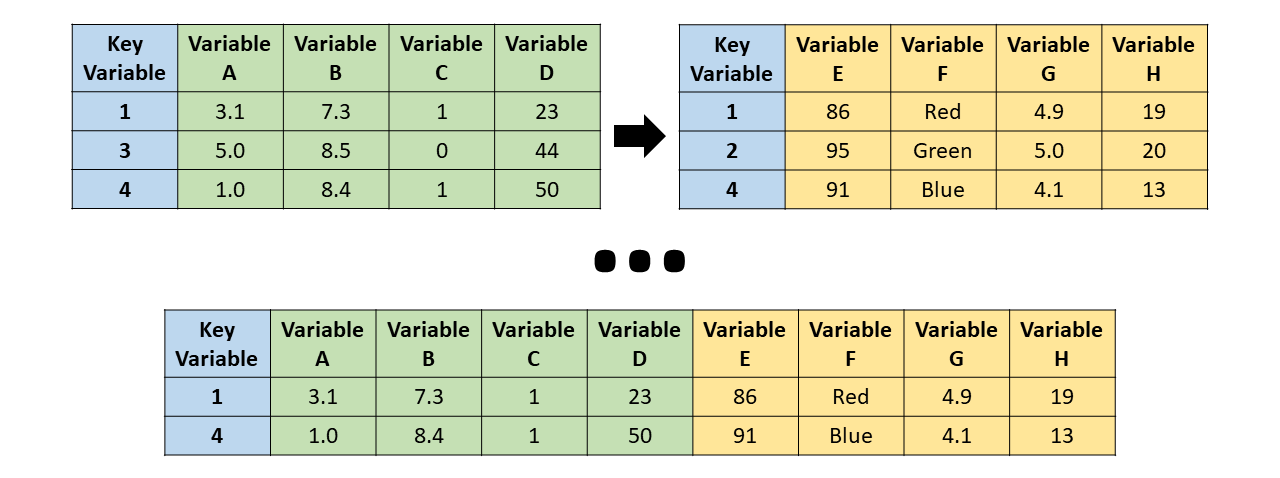
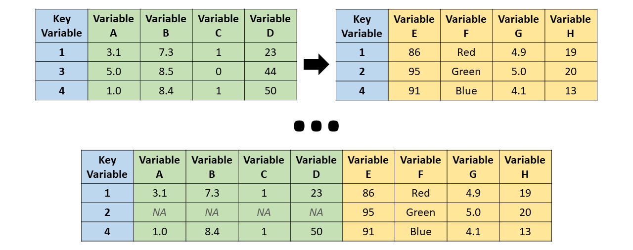
A horizontal join (merge) refers to the process of matching cases (i.e., rows, observations) between two data frames using a key variable (matching variable), which results in distinct sets of variables (i.e., fields, columns) being combined horizontally (laterally) across two data frames. The resulting joined data frame will be wider (in terms of the number of variables) than either of the original data frames in isolation. For example, imagine that we pull data from separate information systems, each with different variables (i.e., fields) but at least some employees (i.e., cases) in common; to combine these two data frames, we can perform a horizontal join. This is often a necessary step when creating a data frame that contains all of the variables we will need in subsequent data analyses. For instance, if we wish to estimate the criterion-related validities using the selection tool scores from one data frame with criterion (e.g., job performance) scores from another data frame, then we could perform a horizontal join, assuming we have a key variable with which to match the scores from the two data frames.
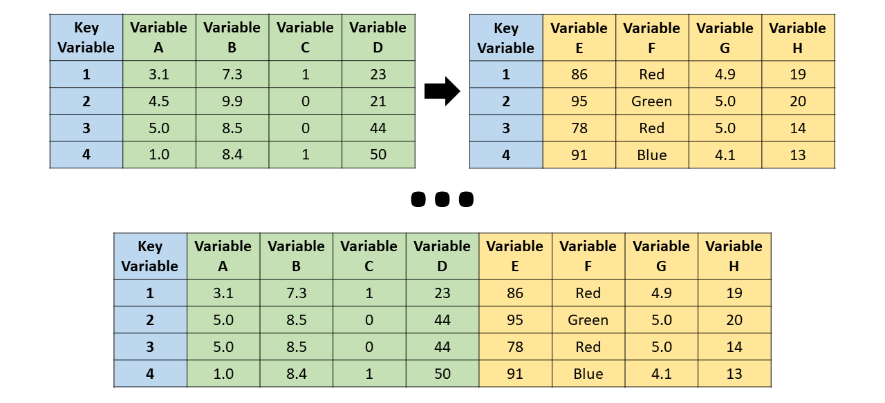
We will focus on four different types of horizontal joins:
- Inner join: All unmatched cases (or observations) are dropped, thereby retaining only those cases that are present in both the left (x, first) and right (y, second) data frames. In other words, a case is only included in the merged data frame if it appears in both of the original data data frames.
- Full join: All cases (or observations) are retained, including those cases that do not have a match in the other data data frame. In other words, a case is included in the merged data frame even if it only appears in one of the original data data frames. These type of join leads to the highest number of retained cases under conditions in which both data frames contain unique cases.
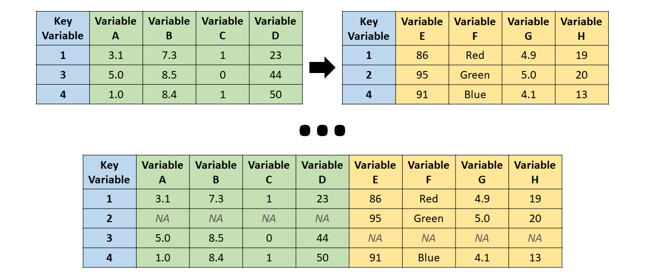
- Left join: All cases (or observations) that appear in the left (x, first) data frame are retained, even if they lack a match in the right (y, second) data frame. Consequently, cases from the right data frame that lack a match in the left data frame are dropped in the merged data frame.
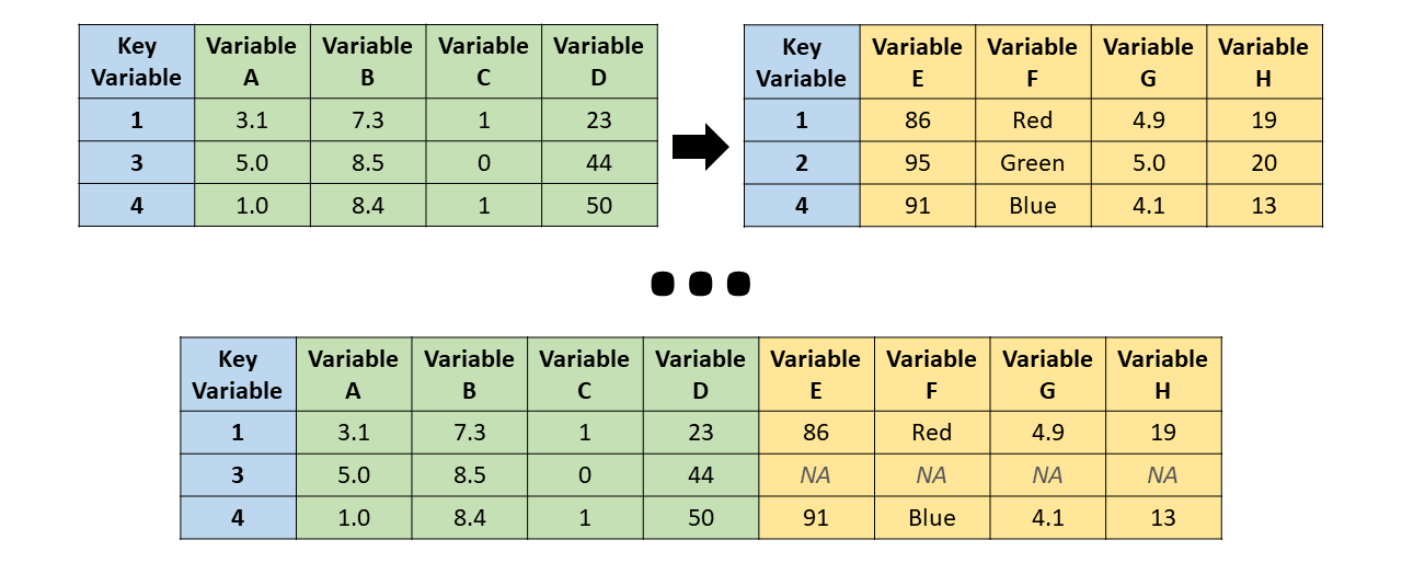
- Right join: All cases (or observations) that appear in the right (y, second) data frame are retained, even if they lack a match in the left (x, first) data frame. Consequently, cases from the left data frame that lack a match in the right data frame are dropped in the merged data frame.
Please note that I have illustrated different types of horizontal joins using a single key variable. It is entirely possible to perform horizontal joins using two or more key variables. For example, imagine that each morning we administered a pulse survey to employees and each afternoon we afternoon we administered a different pulse survey to the same employees, and that we repeated this process for five consecutive workdays. In this instance, we would likely need to horizontally join the data frames using both a unique employee identifier variable and a unique day-of-week variable.
17.1.2 Review of Vertical Joins (Merges)
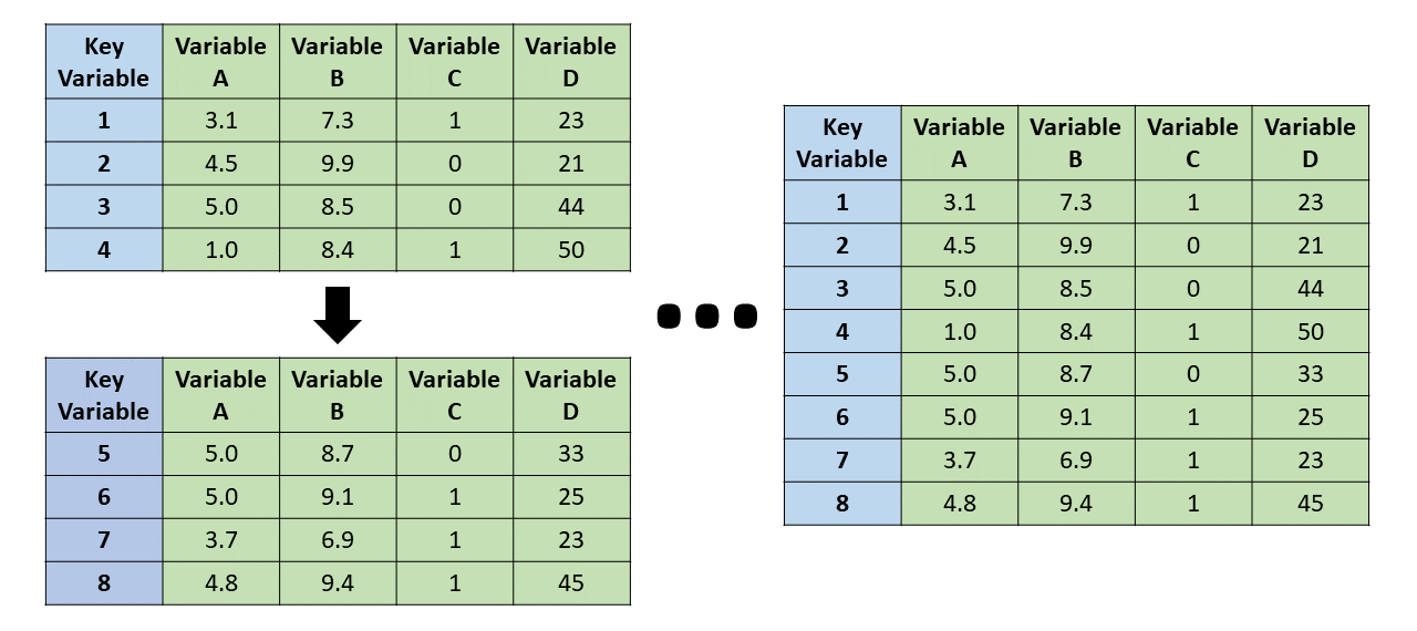
A vertical join (merge) refers to the process of matching identical variables from two data frames, which results in distinct sets of cases or observations being combined vertically. The resulting joined data frame will be longer (in terms of the number of cases) than either of the original data frames in isolation. For example, imagine an organization administered the same survey to two facilities (i.e., independent groups) each with unique employees; we could combine the two resulting data frames by performing a vertical join.
17.2 Tutorial
This chapter’s tutorial demonstrates how to join (merge) cases from two data frames.
17.2.1 Video Tutorial
As usual, you have the choice to follow along with the written tutorial in this chapter or to watch the video tutorial below. Both versions of the tutorial will show you how to join (merge) data with or without the pipe (%>%) operator. If you’re unfamiliar with the pipe operator, no need to worry: I provide a brief explanation and demonstration regarding their purpose in both versions of the tutorial. Finally, please note that in the chapter supplement you have an opportunity to learn how to join (merge) cases from data frames using a function from base R, which you may find preferable or more intuitive.
Link to video tutorial: https://youtu.be/38zsLj-fWo0
17.2.2 Functions & Packages Introduced
| Function | Package |
|---|---|
right_join |
dplyr |
left_join |
dplyr |
inner_join |
dplyr |
full_join |
dplyr |
data.frame |
base R |
c |
base R |
rep |
base R |
rbind |
base R |
17.2.3 Initial Steps
If you haven’t already, save the files called “PersData.csv” and “PerfData.csv” into a folder that you will subsequently set as your working directory. Your working directory will likely be different than the one shown below (i.e., "H:/RWorkshop"). As a reminder, you can access all of the data files referenced in this book by downloading them as a compressed (zipped) folder from the my GitHub site: https://github.com/davidcaughlin/R-Tutorial-Data-Files; once you’ve followed the link to GitHub, just click “Code” (or “Download”) followed by “Download ZIP”, which will download all of the data files referenced in this book. For the sake of parsimony, I recommend downloading all of the data files into the same folder on your computer, which will allow you to set that same folder as your working directory for each of the chapters in this book.
Next, using the setwd function, set your working directory to the folder in which you saved the data files for this chapter. Alternatively, you can manually set your working directory folder in your drop-down menus by going to Session > Set Working Directory > Choose Directory…. Be sure to create a new R script file (.R) or update an existing R script file so that you can save your script and annotations. If you need refreshers on how to set your working directory and how to create and save an R script, please refer to Setting a Working Directory and Creating & Saving an R Script.
Next, read in the .csv data files called “PersData.csv” and “PerfData.csv” using your choice of read function. In this example, I use the read_csv function from the readr package (Wickham, Hester, and Bryan 2024). If you choose to use the read_csv function, be sure that you have installed and accessed the readr package using the install.packages and library functions. Note: You don’t need to install a package every time you wish to access it; in general, I would recommend updating a package installation once ever 1-3 months. For refreshers on installing packages and reading data into R, please refer to Packages and Reading Data into R.
# Install readr package if you haven't already
# [Note: You don't need to install a package every
# time you wish to access it]
install.packages("readr")
# Access readr package
library(readr)
# Read data and name data frame (tibble) objects
personaldata <- read_csv("PersData.csv")## Rows: 9 Columns: 5
## ── Column specification ────────────────────────────────────────────────────────────────────────────────────────────────────────────
## Delimiter: ","
## chr (4): lastname, firstname, startdate, gender
## dbl (1): id
##
## ℹ Use `spec()` to retrieve the full column specification for this data.
## ℹ Specify the column types or set `show_col_types = FALSE` to quiet this message.## Rows: 6 Columns: 5
## ── Column specification ────────────────────────────────────────────────────────────────────────────────────────────────────────────
## Delimiter: ","
## dbl (5): id, perf_q1, perf_q2, perf_q3, perf_q4
##
## ℹ Use `spec()` to retrieve the full column specification for this data.
## ℹ Specify the column types or set `show_col_types = FALSE` to quiet this message.## [1] "id" "lastname" "firstname" "startdate" "gender"## [1] "id" "perf_q1" "perf_q2" "perf_q3" "perf_q4"## # A tibble: 9 × 5
## id lastname firstname startdate gender
## <dbl> <chr> <chr> <chr> <chr>
## 1 153 Sanchez Alejandro 1/1/2016 male
## 2 154 McDonald Ronald 1/9/2016 male
## 3 155 Smith John 1/9/2016 male
## 4 165 Doe Jane 1/4/2016 female
## 5 125 Franklin Benjamin 1/5/2016 male
## 6 111 Newton Isaac 1/9/2016 male
## 7 198 Morales Linda 1/7/2016 female
## 8 201 Providence Cindy 1/9/2016 female
## 9 282 Legend John 1/9/2016 male## # A tibble: 6 × 5
## id perf_q1 perf_q2 perf_q3 perf_q4
## <dbl> <dbl> <dbl> <dbl> <dbl>
## 1 153 3.9 4.8 4.9 5
## 2 125 2.1 1.9 2.1 2.3
## 3 111 3.3 3.3 3.4 3.3
## 4 198 4.9 4.5 4.4 4.8
## 5 201 1.2 1.1 1 1
## 6 282 2.2 2.3 2.4 2.5As you can see from the output generated in your Console, on the one hand, the personaldata data frame object contains basic employee demographic information. The variable names include: id, lastname, firstname, startdate, and gender. On the other hand, the performancedata data frame object contains the same id unique identifier variable as the personaldata data frame object, but instead of employee demographic information, this data frame object includes variables associated with quarterly employee performance: perf_q1, perf_q2, perf_q3, and perf_q4.
In order to better illustrate certain join functions later on in this chapter, we’ll begin by removing the case (i.e., employee) associated with the id variable value of 153 (i.e., Alejandro Sanchez); in terms of a rationale for doing so, let’s imagine that Alejandro no longer works for the organization, and thus we would like to remove him from the personaldata data frame. If you don’t completely understand the following process for removing this individual from the data frame, no need to worry, as you will learn more in the subsequent chapter on filtering data.
- Type the name of the data frame object (
personaldata) followed by the<-operator to overwrite the existing data frame object. - Type the name of the original data frame object (
personaldata) followed by brackets ([ ]). - Within the brackets (
[ ]), type the name of the data frame object (personaldata) again, followed by the$operator and the name of the variable we wish to use to select the case that will be removed, which in this instance is theidunique identifier variable. The$operator indicates to R that theidvariable belongs to thepersonaldatadata frame. - Type the “not equal to” operator, which is
!=(the!means “not”), followed by theidvariable value we wish to use to remove the case (i.e., 153). - Type a comma (
,) to indicate that we are removing a row, not a column. When referencing rows and columns in R, as we are doing in the brackets ([ ]), rows are entered first (before a comma), and columns are entered second (after a comma). In doing so, we are telling R to retain all rows of data inpersonaldataexcept for the one corresponding toidequal to 153.
Check out the first 6 rows of the updated data frame for personaldata, and note that the data corresponding to the case associated with id equal to 153 is gone.
## # A tibble: 6 × 5
##      id lastname firstname startdate gender
##   <dbl> <chr>    <chr>     <chr>     <chr>
## 1   154 McDonald Ronald    1/9/2016  male
## 2   155 Smith    John      1/9/2016  male
## 3   165 Doe      Jane      1/4/2016  female
## 4   125 Franklin Benjamin  1/5/2016  male
## 5   111 Newton   Isaac     1/9/2016  male
## 6   198 Morales  Linda     1/7/2016  female
17.2.4 Horizontal Join (Merge)
Recall that a horizontal join (merge) means that cases are matched using one more more key variables, and as a result, variables (i.e., columns, fields) are combined across two data frames. We will review two options for performing horizontal joins.
To perform horizontal joins, we will learn how to use the join functions from the the dplyr package (Wickham et al. 2023), which include: right_join, left_join, inner_join, and full_join. Please note that there are other functions we could use to perform horizontal joins, and if you’re interested, in the Joining (Merging) Data: Chapter Supplement, I demonstrate how to use the merge function from base R to carry out the same operations we will cover below.
Using the aforementioned join functions, we will match cases from the personaldata and performancedata data frames using the id unique identifier variable as a key variable. So how can we verify that id is an appropriate key variable? Well, let’s use the names function from base R to retrieve the list of variable names from the two data frames, which we already did above. Nevertheless, let’s call up those variable names once more. Simply enter the name of the data frame as a parenthetical argument in the names function.
## [1] "id" "lastname" "firstname" "startdate" "gender"## [1] "id" "perf_q1" "perf_q2" "perf_q3" "perf_q4"As you can see in the variable names listed above, the id variable is common to both data frames, and thus it will serve as our key variable.
Now we are almost ready to begin joining the two data frames using the id unique identifier as a key variable. Before doing so, however, we should make sure that we have installed and accessed the dplyr package (if we haven’t already), as the join functions come from that package.
# Install dplyr package if you haven't already
# [Note: You don't need to install a package every
# time you wish to access it]
install.packages("dplyr")I will demonstrate two techniques for applying the join function.
The first technique uses the pipe operator (%>%). The pipe operator comes from a package called magrittr (Bache and Wickham 2022), on which the dplyr is partially dependent. In short, a pipe allows a person to more efficiently write code and to improve the readability of the code and overall script. Specifically, a pipe forwards the result or value of one object or expression to a subsequent function. In doing so, one can avoid writing functions in which other functions are nested parenthetically. For more information on the pipe operator, check out Wickham and Grolemund’s (2017) chapter on pipes: https://r4ds.had.co.nz/pipes.html.
The second technique for applying the join function takes a more traditional approach in that it involves nested functions being nested parenthetically. If you don’t want to learn how to use pipes (or would like to learn how to use them at a later date), feel free to skip to the section below called Without Pipe.
17.2.4.1 With Pipe
Using the pipe (%>%) operator technique, let’s begin with what is referred to as an inner join by doing the following:
- Use the
<-operator to name the joined (merged) data frame that we will create using the one of thedplyrjoin functions. For this example, I name the new joined data framemergeddf, which is completely arbitrary; you could name it whatever you would like. Make sure you put the name of the new data frame object to the left of the<-operator. - To the right of the
<-operator, type the name of the first data frame, which we namedpersonaldata, followed by the pipe (%>%) operator. This will “pipe” our data frame into the subsequent function. - On the same line or on the next line, type the
inner_joinfunction, and within the parentheses as the first argument, type the name of the second data frame, which we calledperformancedata. As the second argument, use theby=argument to indicate the name of the key variable, which in this example isid; make sure the key variable is in quotation marks (" "), and remember, object and variable names in R are case and space sensitive.
# Inner join (with pipe)
mergeddf <- personaldata %>% inner_join(performancedata, by="id")

# Print the joined data frame
mergeddf
## # A tibble: 5 × 9
## id lastname firstname startdate gender perf_q1 perf_q2 perf_q3 perf_q4
## <dbl> <chr> <chr> <chr> <chr> <dbl> <dbl> <dbl> <dbl>
## 1 125 Franklin Benjamin 1/5/2016 male 2.1 1.9 2.1 2.3
## 2 111 Newton Isaac 1/9/2016 male 3.3 3.3 3.4 3.3
## 3 198 Morales Linda 1/7/2016 female 4.9 4.5 4.4 4.8
## 4 201 Providence Cindy 1/9/2016 female 1.2 1.1 1 1
## 5 282 Legend John 1/9/2016 male 2.2 2.3 2.4 2.5Now, let’s revisit the original data frame objects that we read in initially.
## # A tibble: 8 × 5
##      id lastname   firstname startdate gender
##   <dbl> <chr>      <chr>     <chr>     <chr>
## 1   154 McDonald   Ronald    1/9/2016  male
## 2   155 Smith      John      1/9/2016  male
## 3   165 Doe        Jane      1/4/2016  female
## 4   125 Franklin   Benjamin  1/5/2016  male
## 5   111 Newton     Isaac     1/9/2016  male
## 6   198 Morales    Linda     1/7/2016  female
## 7   201 Providence Cindy     1/9/2016  female
## 8 282 Legend John 1/9/2016 male## # A tibble: 6 × 5
## id perf_q1 perf_q2 perf_q3 perf_q4
## <dbl> <dbl> <dbl> <dbl> <dbl>
## 1 153 3.9 4.8 4.9 5
## 2 125 2.1 1.9 2.1 2.3
## 3 111 3.3 3.3 3.4 3.3
## 4 198 4.9 4.5 4.4 4.8
## 5 201 1.2 1.1 1 1
## 6 282 2.2 2.3 2.4 2.5In the output, first, note how all of the variables from the original data frames (i.e., personaldata, performancedata) are represented in the merged data frame (i.e., mergeddf). Second, note how the cases are matched by the id key variable. Third, note that the personaldata data frame has 8 cases, the performancedata data frame has 6 cases, and the mergeddf data frame has 6 cases. By default, the merge function performs an inner join and retains only those matched cases that have data in both data frames. Because cases whose id values were 154, 155, and 165 had data in personaldata but not performancedata and because the case with an id value equal to 153 was in performancedata but not personaldata, only the 5 cases that had available data in both data frames were retained.
To perform what is referred to as a full join in which we retain all cases and available data, we simply swap out the inner_join function from our previous code with the full_join function.
# Full join (with pipe)
mergeddf <- personaldata %>% full_join(performancedata, by="id")

# Print the joined data frame
mergeddf
## # A tibble: 9 × 9
## id lastname firstname startdate gender perf_q1 perf_q2 perf_q3 perf_q4
## <dbl> <chr> <chr> <chr> <chr> <dbl> <dbl> <dbl> <dbl>
## 1 154 McDonald Ronald 1/9/2016 male NA NA NA NA
## 2 155 Smith John 1/9/2016 male NA NA NA NA
## 3 165 Doe Jane 1/4/2016 female NA NA NA NA
## 4 125 Franklin Benjamin 1/5/2016 male 2.1 1.9 2.1 2.3
## 5 111 Newton Isaac 1/9/2016 male 3.3 3.3 3.4 3.3
## 6 198 Morales Linda 1/7/2016 female 4.9 4.5 4.4 4.8
## 7 201 Providence Cindy 1/9/2016 female 1.2 1.1 1 1
## 8 282 Legend John 1/9/2016 male 2.2 2.3 2.4 2.5
## 9 153 <NA> <NA> <NA> <NA> 3.9 4.8 4.9 5Note how the full_join function retains all available cases that had available data in at least one of the data frames, which in this example is 9 cases. When in doubt, I recommend using the full_join function to retain all available data.
To perform what is referred to as a left join in which we retain only those cases with data available in the first (left, x) data frame (personaldata), we use the left_join function instead, while keeping the rest of the previous code the same.
# Left join (with pipe)
mergeddf <- personaldata %>% left_join(performancedata, by="id")

# Print the joined data frame
mergeddf
## # A tibble: 8 × 9
## id lastname firstname startdate gender perf_q1 perf_q2 perf_q3 perf_q4
## <dbl> <chr> <chr> <chr> <chr> <dbl> <dbl> <dbl> <dbl>
## 1 154 McDonald Ronald 1/9/2016 male NA NA NA NA
## 2 155 Smith John 1/9/2016 male NA NA NA NA
## 3 165 Doe Jane 1/4/2016 female NA NA NA NA
## 4 125 Franklin Benjamin 1/5/2016 male 2.1 1.9 2.1 2.3
## 5 111 Newton Isaac 1/9/2016 male 3.3 3.3 3.4 3.3
## 6 198 Morales Linda 1/7/2016 female 4.9 4.5 4.4 4.8
## 7 201 Providence Cindy 1/9/2016 female 1.2 1.1 1 1
## 8 282 Legend John 1/9/2016 male 2.2 2.3 2.4 2.5Note how the left_join function retains only those cases for which the first (left, x) data frame (i.e., personaldata) has complete data, which in this case happens to be 8 cases. Notably absent is the case associated with id equal to 153 because the first (left, x) data frame (i.e., personaldata) lacked that case. An NA appears for each case from the second (right, y) data frame that contained missing values on variables from that data frame.
To perform what is referred to as a right join in which we retain only those cases with data available in the second (right, y) data frame (performancedata), we will use the right_join function instead, while keeping the rest of the previous code the same.
# Right join (with pipe)
mergeddf <- personaldata %>% right_join(performancedata, by="id")

# Print the joined data frame
mergeddf
## # A tibble: 6 × 9
## id lastname firstname startdate gender perf_q1 perf_q2 perf_q3 perf_q4
## <dbl> <chr> <chr> <chr> <chr> <dbl> <dbl> <dbl> <dbl>
## 1 125 Franklin Benjamin 1/5/2016 male 2.1 1.9 2.1 2.3
## 2 111 Newton Isaac 1/9/2016 male 3.3 3.3 3.4 3.3
## 3 198 Morales Linda 1/7/2016 female 4.9 4.5 4.4 4.8
## 4 201 Providence Cindy 1/9/2016 female 1.2 1.1 1 1
## 5 282 Legend John 1/9/2016 male 2.2 2.3 2.4 2.5
## 6 153 <NA> <NA> <NA> <NA> 3.9 4.8 4.9 5Note how the right_join function retains only those cases for which the joined (second, right, y) data frame (i.e., performancedata) has complete data. Because the first (left, x) data frame lacks data for the case in which id is equal to 153, an NA appears for each case from the first data frame that contained missing values on variables from that data frame.
17.2.4.2 Without Pipe
In this section, I demonstrate the same dplyr join functions as above, except here I demonstrate how to specify the functions without the use of a pipe (%>%) operator.
Let’s begin with what is referred to as an inner join by doing the following:
- Use the
<-operator to name the joined (merged) data frame that we will create using the one of thedplyrjoin functions. For this example, I name the new joined data framemergeddf, which is completely arbitrary; you could name it whatever you would like. Make sure you put the name of the new data frame object to the left of the<-operator. - To the right of the
<-operator, type the name of theinner_joinfunction. As the first argument within the parentheses, type the name of the first data frame, which we namedpersonaldata. As the second argument, type the name of the second data frame we namedperformancedata. As the third argument, use theby=argument to indicate the name of the key variable, which in this example isid; make sure the key variable is in quotation marks (" "), and remember, object and variable names in R are case and space sensitive.
# Inner join (without pipe)
mergeddf <- inner_join(personaldata, performancedata, by="id")

# Print the joined data frame
mergeddf
## # A tibble: 5 × 9
## id lastname firstname startdate gender perf_q1 perf_q2 perf_q3 perf_q4
## <dbl> <chr> <chr> <chr> <chr> <dbl> <dbl> <dbl> <dbl>
## 1 125 Franklin Benjamin 1/5/2016 male 2.1 1.9 2.1 2.3
## 2 111 Newton Isaac 1/9/2016 male 3.3 3.3 3.4 3.3
## 3 198 Morales Linda 1/7/2016 female 4.9 4.5 4.4 4.8
## 4 201 Providence Cindy 1/9/2016 female 1.2 1.1 1 1
## 5 282 Legend John 1/9/2016 male 2.2 2.3 2.4 2.5Now, let’s revisit the original data frame objects that we read in initially.
## # A tibble: 8 × 5
##      id lastname   firstname startdate gender
##   <dbl> <chr>      <chr>     <chr>     <chr>
## 1   154 McDonald   Ronald    1/9/2016  male
## 2   155 Smith      John      1/9/2016  male
## 3   165 Doe        Jane      1/4/2016  female
## 4   125 Franklin   Benjamin  1/5/2016  male
## 5   111 Newton     Isaac     1/9/2016  male
## 6   198 Morales    Linda     1/7/2016  female
## 7   201 Providence Cindy     1/9/2016  female
## 8 282 Legend John 1/9/2016 male## # A tibble: 6 × 5
## id perf_q1 perf_q2 perf_q3 perf_q4
## <dbl> <dbl> <dbl> <dbl> <dbl>
## 1 153 3.9 4.8 4.9 5
## 2 125 2.1 1.9 2.1 2.3
## 3 111 3.3 3.3 3.4 3.3
## 4 198 4.9 4.5 4.4 4.8
## 5 201 1.2 1.1 1 1
## 6 282 2.2 2.3 2.4 2.5In the output, first, note how all of the variables from the original data frames (i.e., personaldata, performancedata) are represented in the merged data frame (i.e., mergeddf). Second, note how the cases are matched by the id key variable. Third, note that the personaldata data frame has 8 cases, the performancedata data frame has 6 cases, and the mergeddf data frame has 6 cases. By default, the merge function performs an inner join and retains only those matched cases that have data in both data frames. Because cases whose id values were 154, 155, and 165 had data in personaldata but not performancedata and because the case with an id value equal to 153 was in performancedata but not personaldata, only the 5 cases that had available data in both data frames were retained.
To perform what is referred to as a full join in which we retain all cases and available data, we simply swap out the inner_join function from our previous code with the full_join function.
# Full join (without pipe)
mergeddf <- full_join(personaldata, performancedata, by="id")

# Print the joined data frame
mergeddf
## # A tibble: 9 × 9
## id lastname firstname startdate gender perf_q1 perf_q2 perf_q3 perf_q4
## <dbl> <chr> <chr> <chr> <chr> <dbl> <dbl> <dbl> <dbl>
## 1 154 McDonald Ronald 1/9/2016 male NA NA NA NA
## 2 155 Smith John 1/9/2016 male NA NA NA NA
## 3 165 Doe Jane 1/4/2016 female NA NA NA NA
## 4 125 Franklin Benjamin 1/5/2016 male 2.1 1.9 2.1 2.3
## 5 111 Newton Isaac 1/9/2016 male 3.3 3.3 3.4 3.3
## 6 198 Morales Linda 1/7/2016 female 4.9 4.5 4.4 4.8
## 7 201 Providence Cindy 1/9/2016 female 1.2 1.1 1 1
## 8 282 Legend John 1/9/2016 male 2.2 2.3 2.4 2.5
## 9 153 <NA> <NA> <NA> <NA> 3.9 4.8 4.9 5Note how the full_join function retains all available cases that had available data in at least one of the data frames, which in this example is 9 cases. When in doubt, I recommend using the full_join function to retain all available data.
To perform what is referred to as a left join in which we retain only those cases with data available in the first (left, x) data frame (personaldata), we use the left_join function instead, while keeping the rest of the previous code the same.
# Left join (without pipe)
mergeddf <- left_join(personaldata, performancedata, by="id")

# Print the joined data frame
mergeddf
## # A tibble: 8 × 9
## id lastname firstname startdate gender perf_q1 perf_q2 perf_q3 perf_q4
## <dbl> <chr> <chr> <chr> <chr> <dbl> <dbl> <dbl> <dbl>
## 1 154 McDonald Ronald 1/9/2016 male NA NA NA NA
## 2 155 Smith John 1/9/2016 male NA NA NA NA
## 3 165 Doe Jane 1/4/2016 female NA NA NA NA
## 4 125 Franklin Benjamin 1/5/2016 male 2.1 1.9 2.1 2.3
## 5 111 Newton Isaac 1/9/2016 male 3.3 3.3 3.4 3.3
## 6 198 Morales Linda 1/7/2016 female 4.9 4.5 4.4 4.8
## 7 201 Providence Cindy 1/9/2016 female 1.2 1.1 1 1
## 8 282 Legend John 1/9/2016 male 2.2 2.3 2.4 2.5Note how the left_join function retains only those cases for which the first (left, x) data frame (i.e., personaldata) has complete data, which in this case happens to be 8 cases. Notably absent is the case associated with id equal to 153 because the first (left, x) data frame (i.e., personaldata) lacked that case. An NA appears for each case from the second (right, y) data frame that contained missing values on variables from that data frame.
To perform what is referred to as a right join in which we retain only those cases with data available in the second (right, y) data frame (performancedata), we use the right_join function instead, while keeping the rest of the previous code the same.
# Right join (without pipe)
mergeddf <- right_join(personaldata, performancedata, by="id")

# Print the joined data frame
mergeddf
## # A tibble: 6 × 9
## id lastname firstname startdate gender perf_q1 perf_q2 perf_q3 perf_q4
## <dbl> <chr> <chr> <chr> <chr> <dbl> <dbl> <dbl> <dbl>
## 1 125 Franklin Benjamin 1/5/2016 male 2.1 1.9 2.1 2.3
## 2 111 Newton Isaac 1/9/2016 male 3.3 3.3 3.4 3.3
## 3 198 Morales Linda 1/7/2016 female 4.9 4.5 4.4 4.8
## 4 201 Providence Cindy 1/9/2016 female 1.2 1.1 1 1
## 5 282 Legend John 1/9/2016 male 2.2 2.3 2.4 2.5
## 6 153 <NA> <NA> <NA> <NA> 3.9 4.8 4.9 5Note how the right_join function retains only those cases for which the joined (second, right, y) data frame (i.e., performancedata) has complete data. Because the first (left, x) data frame lacks data for the case in which id is equal to 153, an NA appears for each case from the first data frame that contained missing values on variables from that data frame.
17.2.5 Vertical Join (Merge)
To perform a vertical join (merge), we will use the rbind function from base R, which stands for “row bind.” As a reminder, with a horizontal join, our focus is on joining variables (i.e., columns, fields) from two data frames containing overlapping cases (i.e., rows). In contrast, with a vertical join, our focus is on joining cases from data frames with the same variables.
To illustrate how to perform a vertical join, we take a slightly different approach than what we did with horizontal joins. Instead of reading in data files, we will create two “toy” employee demographic data frames with the exact same variables but different cases. We will use the data.frame function from base R to indicate that we wish to create a data frame object; we use the c (combine) function from base R to combine values into a vector; and we use the rep (replicate) function from base R to replicate the same value a specified number of times. Also note that the : operator, when used between two numbers, creates a vector of consecutive values, beginning with the first value and ending with the second. Please note, that using and understanding the data.frame, c, and rep functions is not consequential for understanding how to do a vertical merge; rather, I merely use these functions in this tutorial to create quick toy data frames that we can use to illustrate how to do a vertical join. For more information on the data.frame function and the c function, please refer to the chapter called Basic Features and Operations of the R Language.
# Create data frames with same variables but arbitrary values
df1 <- data.frame(id=c(1:6), age=c(21:26), sex=c(rep("male", 6)))
df2 <- data.frame(id=c(7:10), age=c(27:30), sex=c(rep("female", 4)))## id age sex
## 1 1 21 male
## 2 2 22 male
## 3 3 23 male
## 4 4 24 male
## 5 5 25 male
## 6 6 26 male## id age sex
## 1 7 27 female
## 2 8 28 female
## 3 9 29 female
## 4 10 30 femaleGiven that these two data frames (i.e., df1, df2) have the exact same variable names (id, age, and sex), we can easily perform a vertical join using the rbind function. To do so, enter the names of the two data frames as arguments, separated by a comma. Use the <- operator to name the merged data frame something, which for this case, I arbitrarily named it mergeddf2.
##   id age  sex
## 1  1  21 male
## 2  2  22 male
## 3  3  23 male
## 4  4  24 male
## 5  5  25 male
## 6  6  26 male
## 7 7 27 female
## 8 8 28 female
## 9 9 29 female
## 10 10 30 femaleNote how the two data frames are now “stacked” on one another. This was possible because they shared the same variables names and variables types (e.g., numeric and character).
17.2.6 Summary
Joining (merging) data frames in R is a useful practice. In this chapter, we learned how to perform a horizontal join using the right_join, left_join, inner_join, and full_join functions from the dplyr package. We also learned how to perform a vertical join using the rbind function from base R.
17.3 Chapter Supplement
In addition to the join functions from the dplyr package covered above, we can use the merge function from base R to perform a horizontal join. Because this function comes from base R, we do not need to install and access an additional package like we do with the join functions, which some may find advantageous.
17.3.1 Video Tutorial
In addition to the written chapter supplement provided below, you can follow along with the following video tutorial to learn more about how to horizontally join data two data frames using the merge function from base R.
Link to video tutorial: https://youtu.be/MLihEVEpJBg
17.3.3 Initial Steps
If required, please refer to the Initial Steps section from this chapter for more information on these initial steps. Please note, however, that we are using two slightly different data files in this supplement, which will simply and clarify some of the different types of merges (joins) that we’ll go over.
# Access readr package
library(readr)

# Read data and name data frame (tibble) objects
# Note that these data files are different than the
# ones we used in the main part of the chapter
personaldata <- read_csv("PersonalData.csv")
## Rows: 8 Columns: 5
## ── Column specification ────────────────────────────────────────────────────────────────────────────────────────────────────────────
## Delimiter: ","
## chr (4): lastname, firstname, startdate, gender
## dbl (1): id
##
## ℹ Use `spec()` to retrieve the full column specification for this data.
## ℹ Specify the column types or set `show_col_types = FALSE` to quiet this message.## Rows: 6 Columns: 5
## ── Column specification ────────────────────────────────────────────────────────────────────────────────────────────────────────────
## Delimiter: ","
## dbl (5): id, perf_q1, perf_q2, perf_q3, perf_q4
##
## ℹ Use `spec()` to retrieve the full column specification for this data.
## ℹ Specify the column types or set `show_col_types = FALSE` to quiet this message.## [1] "id" "lastname" "firstname" "startdate" "gender"## [1] "id" "perf_q1" "perf_q2" "perf_q3" "perf_q4"## # A tibble: 8 × 5
## id lastname firstname startdate gender
## <dbl> <chr> <chr> <chr> <chr>
## 1 153 Sanchez Alejandro 1/1/2016 man
## 2 154 McDonald Ronald 1/9/2016 man
## 3 155 Smith John 1/9/2016 man
## 4 165 Doe Jane 1/4/2016 woman
## 5 111 Newton Isaac 1/9/2016 man
## 6 198 Morales Linda 1/7/2016 woman
## 7 201 Providence Cindy 1/9/2016 woman
## 8 282 Legend John 1/9/2016 man## # A tibble: 6 × 5
## id perf_q1 perf_q2 perf_q3 perf_q4
## <dbl> <dbl> <dbl> <dbl> <dbl>
## 1 153 3.9 4.8 4.9 5
## 2 125 2.1 1.9 2.1 2.3
## 3 111 3.3 3.3 3.4 3.3
## 4 198 4.9 4.5 4.4 4.8
## 5 201 1.2 1.1 1 1
## 6 282 2.2 2.3 2.4 2.517.3.4 merge Function from Base R
We will use the merge function to horizontally match cases from the personaldata and performancedata data frames using id as a key variable. To identify what the key variable is, let’s use the names function from base R to print the list of variable names from the two data frames, which we already did above. Nevertheless, let’s call up those variable names once more. Simply enter the name of the data frame as a parenthetical argument in the names function.
## [1] "id" "lastname" "firstname" "startdate" "gender"## [1] "id" "perf_q1" "perf_q2" "perf_q3" "perf_q4"As you can see in the variable names listed above, the id variable is common to both data frames, and thus it will serve as our key variable.
Let’s begin with what is referred to as an inner join:
- Use the
<-operator to name the joined data frame that we create using themergefunction. For this example, I name the new joined data framemergeddf, which is completely arbitrary; you could name it whatever you would like. Type the name of the new joined data frame to the left of the<-operator. - To the right of the
<-operator, type the name of themergefunction. Within themergefunction parentheses, we will provide the arguments needed to make this join a reality. First, enter the name of one of the data frames (e.g.,personaldata), followed by a comma. Second, enter the name of of the other data frame (e.g.,performancedata), followed by a comma. Third, use theby=argument to indicate the name of the key variable (e.g.,id); make sure the key variable is in quotation marks (" "), and remember, object and variable names in R are case and space sensitive.
# Inner join
mergeddf <- merge(personaldata, performancedata, by="id")
# Print the joined data frame
mergeddf## id lastname firstname startdate gender perf_q1 perf_q2 perf_q3 perf_q4
## 1 111 Newton Isaac 1/9/2016 man 3.3 3.3 3.4 3.3
## 2 153 Sanchez Alejandro 1/1/2016 man 3.9 4.8 4.9 5.0
## 3 198 Morales Linda 1/7/2016 woman 4.9 4.5 4.4 4.8
## 4 201 Providence Cindy 1/9/2016 woman 1.2 1.1 1.0 1.0
## 5 282 Legend John 1/9/2016 man 2.2 2.3 2.4 2.5Now, let’s revisit the original data frame objects that we read in initially.
## # A tibble: 8 × 5
##      id lastname   firstname startdate gender
##   <dbl> <chr>      <chr>     <chr>     <chr>
## 1   153 Sanchez    Alejandro 1/1/2016  man
## 2   154 McDonald   Ronald    1/9/2016  man
## 3   155 Smith      John      1/9/2016  man
## 4   165 Doe        Jane      1/4/2016  woman
## 5   111 Newton     Isaac     1/9/2016  man
## 6   198 Morales    Linda     1/7/2016  woman
## 7   201 Providence Cindy     1/9/2016  woman
## 8 282 Legend John 1/9/2016 man## # A tibble: 6 × 5
## id perf_q1 perf_q2 perf_q3 perf_q4
## <dbl> <dbl> <dbl> <dbl> <dbl>
## 1 153 3.9 4.8 4.9 5
## 2 125 2.1 1.9 2.1 2.3
## 3 111 3.3 3.3 3.4 3.3
## 4 198 4.9 4.5 4.4 4.8
## 5 201 1.2 1.1 1 1
## 6 282 2.2 2.3 2.4 2.5In the output, first, note how all of the variables from the original data frames (i.e., personaldata, performancedata) are represented in the merged data frame (i.e., mergeddf). Second, note how the cases are matched by the id key variable. Third, note that the personaldata data frame has 8 cases, the performancedata data frame has 6 cases, and the mergeddf data frame has 6 cases. By default, the merge function performs an inner join and retains only those matched cases that have data in both data frames. Because cases whose id values were 154, 155, and 165 had data in personaldata but not performancedata and because the case with an id value equal to 153 was in performancedata but not personaldata, only the 5 cases that had available data in both data frames were retained.
To perform what is referred to as a full join in which we retain all cases and available data, we can add the all= argument to our previous code and specify the logical value TRUE.
# Full join
mergeddf <- merge(personaldata, performancedata, by="id", all=TRUE)

# Print the joined data frame
mergeddf
## id lastname firstname startdate gender perf_q1 perf_q2 perf_q3 perf_q4
## 1 111 Newton Isaac 1/9/2016 man 3.3 3.3 3.4 3.3
## 2 125 <NA> <NA> <NA> <NA> 2.1 1.9 2.1 2.3
## 3 153 Sanchez Alejandro 1/1/2016 man 3.9 4.8 4.9 5.0
## 4 154 McDonald Ronald 1/9/2016 man NA NA NA NA
## 5 155 Smith John 1/9/2016 man NA NA NA NA
## 6 165 Doe Jane 1/4/2016 woman NA NA NA NA
## 7 198 Morales Linda 1/7/2016 woman 4.9 4.5 4.4 4.8
## 8 201 Providence Cindy 1/9/2016 woman 1.2 1.1 1.0 1.0
## 9 282 Legend John 1/9/2016 man 2.2 2.3 2.4 2.5Note how the full_join function retains all available cases that had available data in at least one of the data frames, which in this example is 9 cases. When in doubt, I recommend using the full_join function to retain all available data.
To perform what is referred to as a left join in which we retain only those cases with data available in the first (left, x) data frame (personaldata), we use the all.x=TRUE argument instead.
# Left join
mergeddf <- merge(personaldata, performancedata, by="id", all.x=TRUE)

# Print the joined data frame
mergeddf
## id lastname firstname startdate gender perf_q1 perf_q2 perf_q3 perf_q4
## 1 111 Newton Isaac 1/9/2016 man 3.3 3.3 3.4 3.3
## 2 153 Sanchez Alejandro 1/1/2016 man 3.9 4.8 4.9 5.0
## 3 154 McDonald Ronald 1/9/2016 man NA NA NA NA
## 4 155 Smith John 1/9/2016 man NA NA NA NA
## 5 165 Doe Jane 1/4/2016 woman NA NA NA NA
## 6 198 Morales Linda 1/7/2016 woman 4.9 4.5 4.4 4.8
## 7 201 Providence Cindy 1/9/2016 woman 1.2 1.1 1.0 1.0
## 8 282 Legend John 1/9/2016 man 2.2 2.3 2.4 2.5Note how the left join retains only those cases for which the first (left, x) data frame (i.e., personaldata) has complete data, which in this case happens to be 8 cases. Notably absent is the case associated with id equal to 153 because the first (left, x) data frame (i.e., personaldata) lacked that case. An NA appears for each case from the second (right, y) data frame that contained missing values on variables from that data frame.
To perform what is referred to as a right join in which we retain only those cases with data available in the second (right, y) data frame (performancedata), we use the all.y=TRUE argument instead.
# Right join
mergeddf <- merge(personaldata, performancedata, by="id", all.y=TRUE)

# Print the joined data frame
mergeddf
## id lastname firstname startdate gender perf_q1 perf_q2 perf_q3 perf_q4
## 1 111 Newton Isaac 1/9/2016 man 3.3 3.3 3.4 3.3
## 2 125 <NA> <NA> <NA> <NA> 2.1 1.9 2.1 2.3
## 3 153 Sanchez Alejandro 1/1/2016 man 3.9 4.8 4.9 5.0
## 4 198 Morales Linda 1/7/2016 woman 4.9 4.5 4.4 4.8
## 5 201 Providence Cindy 1/9/2016 woman 1.2 1.1 1.0 1.0
## 6 282 Legend John 1/9/2016 man 2.2 2.3 2.4 2.5Note how the right join retains only those cases for which the joined (second, right, y) data frame (i.e., performancedata) has complete data. Because the first (left, x) data frame lacks data for the case in which id is equal to 153, an NA appears for each case from the first data frame that contained missing values on variables from that data frame.