Chapter 49 Applying k-Fold Cross-Validation to Logistic Regression
In this chapter, we will learn how to apply k-fold cross-validation to logistic regression. As a specific type of cross-validation, k-fold cross-validation can be a useful framework for training and testing models.
49.1 Conceptual Overview
In general, cross-validation is an integral part of predictive analytics, as it allows us to understand how a model estimated on one data set will perform when applied to one or more new data sets. Cross-validation was initially introduced in the chapter on statistically and empirically cross-validating a selection tool using multiple linear regression. k-fold cross-validation is a specific type of cross-validation that is commonly applied when carrying out predictive analytics.
49.1.1 Review of Predictive Analytics
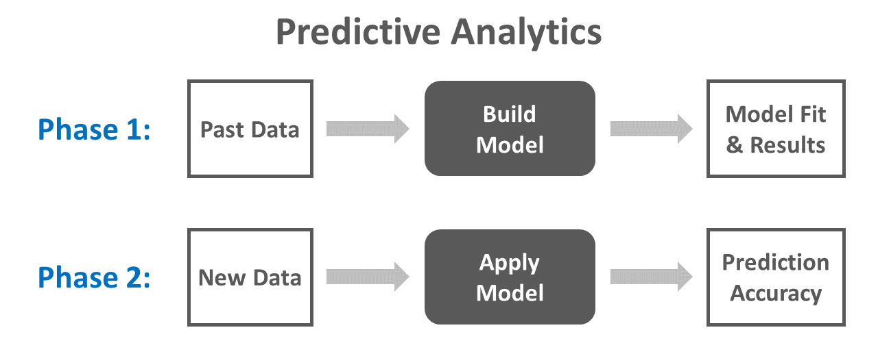
True predictive analytics involves training (i.e., estimating, building) a model using one or more samples of data and then evaluating (i.e., testing, validating) how well the model performs when applied to a separate sample of data drawn from the same population. Assuming we have a large enough data set to begin with, we often assign 80% of the cases to a training data set and 20% to a test data set. The term predictive analytics is a big umbrella term, and predictive analytics can be applied using many different types of models, including common regression model types like ordinary least squares (OLS) multiple linear regression or maximum likelihood logistic regression. When building a model using a predictive analytics framework, one of our goals is to minimize prediction errors (i.e., improve prediction accuracy) when the model is applied to “fresh” or “new” data (e.g., test data). Fewer prediction errors when applying the model to new data indicate that the model makes more accurate predictions. At the same time, we want to avoid overfitting our model to the data on which it is trained, as this can lead to a model that fits our training data well but that doesn’t generalize to our test data; applying a trained model to new data can help us evaluate the extent to which we might have overfit a model to the original data. Fortunately, there are multiple cross-validation frameworks that we can apply when training a model, and these frameworks can help us improve a model’s predictive performance/accuracy while also reducing the occurrence of overfitting. One such cross-validation framework is k-fold cross-validation.
49.1.2 Review of k-Fold Cross-Validation
Often, when applying a predictive analytics process, we do some sort of variation of the two-phase process described above: (a) train the model on one set of data, and (b) test the model on a separate set of data. We typically put a lot of thought and consideration into how to train a model using the training data. Not only do we need to identify an appropriate type of statistical model, but we also need to consider whether we will incorporate validation into the model-training process. A common validation approach is k-fold cross-validation. To perform k-fold cross-validation, we often do the following:
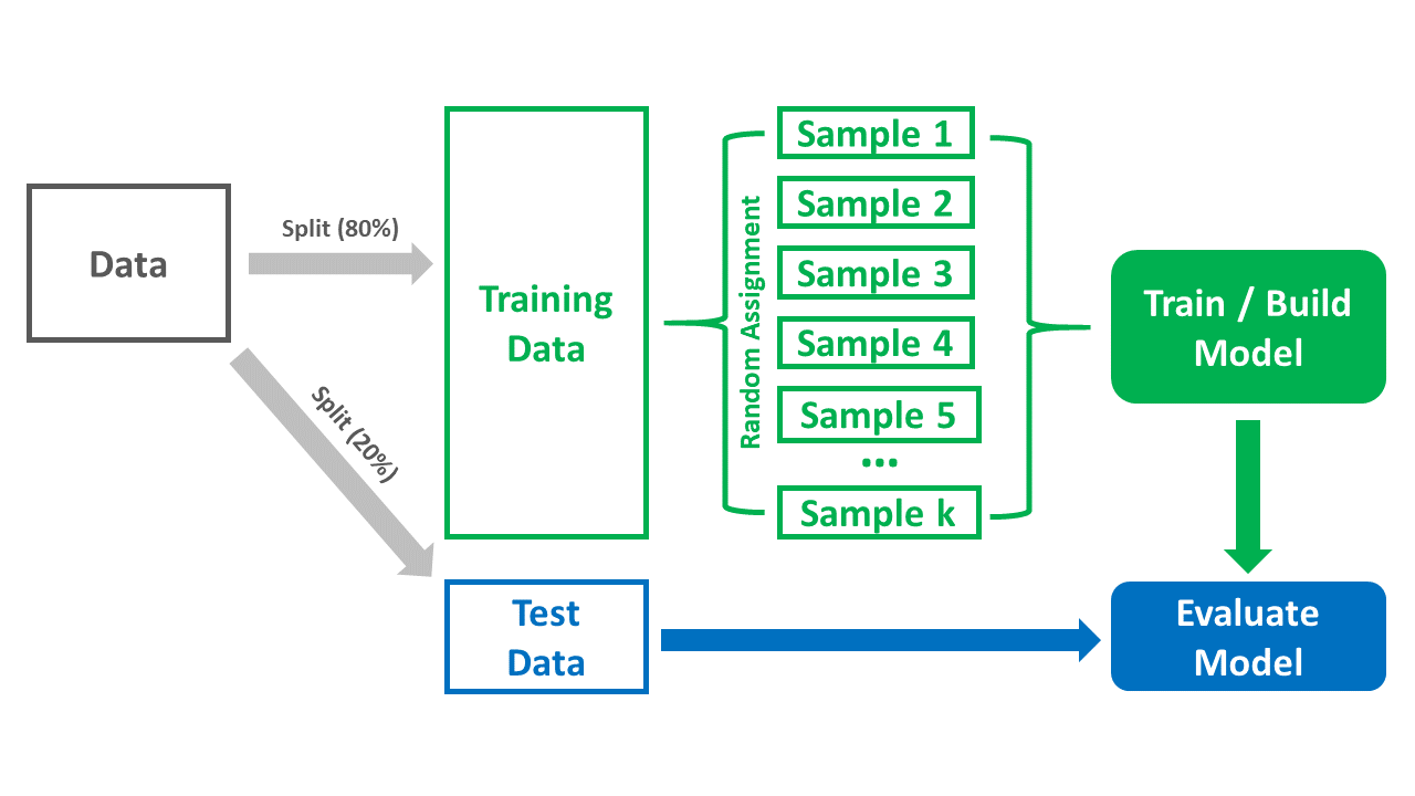
- We split the data into a training data set and a test data set. Commonly, 80% of the data are randomly selected for the training data set, while the remaining 20% end up in the test data set.
- We randomly split the training data into two or more (sub)samples, which will allow us to train the model in an iterative process. The total number of samples we split the data into will be equal to k, where k refers to the number of folds (i.e., resamples). For example, if we randomly split the training data into five samples, then our k will be 5, and thus we will be performing 5-fold cross-validation. We then use the k samples to train (i.e., estimate, build) our model, which is accomplished through iterating the model-estimation process across k folds of data. For each fold, we estimate the model based on pooled data from k-1 samples. That is, if we split our training data into 5 samples, then for the first fold we might estimate the model based on data pooled together from the first four samples (out of five); we then use the fifth “holdout” (i.e., kth) sample as the validation sample, which means we assess the estimated model’s predictive performance/accuracy on data that weren’t used for that specific model estimation process. This process repeats until every sample has served as the validation sample, for a total of k folds. The models’ estimated performance across the k folds is then synthesized. Specifically, the k cross-validated models are then tossed out, but the estimated error from those models can be synthesized (e.g., averaged) to arrive at a performance estimate for the final model. With some types of models, the estimated error (e.g., root mean-squared error, R2) from those models is used to inform the final model estimation. Note that the final model’s parameter estimates are typically estimated using all of the available training data.
- The k-fold cross-validation framework can be extended by taking the final trained model and evaluating its performance based on the test data set that – to this point – has yet to be used; this is how k-fold cross-validation can be used in a broader predictive analytics (i.e., predictive modeling) context. It is important to note, however, that there are other cross-validation approaches we might choose, such as traditional empirical cross-validation (holdout method) and leave-one-out cross-validation (LOOCV) – but those are beyond the scope of this chapter. James, Witten, Hastie, and Tibshirani (2013) provide a nice introduction to LOOCV; though, in short, LOOCV is a specific instance of k-fold cross-validation in which k is equal to the number of observations in the training data. The figure below provides a visual overview of the k-fold cross-validation process, which we will bring to life in the tutorial portion of this chapter.
In this chapter, we will focus on applying k-fold cross-validation to the estimation and evaluation of a multiple logistic regression model. The use of logistic regression implies that our outcome variable will be dichotomous. For background information on logistic regression, including the statistical assumptions that should be satisfied, check out the prior chapter on logistic regression. I must note, however, that other types of statistical models can be applied within a k-fold cross-validation framework – or any cross-validation framework for that matter. For example, assuming the appropriate statistical assumptions have been met, we might also apply more traditional regression-based approaches like ordinary least squares (OLS) multiple linear regression, or we could apply supervised statistical learning models like Lasso regression, which will be covered in a later chapter.
49.1.3 Conceptual Video
For a more in-depth review of k-fold cross-validation, please check out the following conceptual video.
Link to conceptual video: https://youtu.be/kituDjzXwfE
49.2 Tutorial
This chapter’s tutorial demonstrates how to estimate and evaluate a multiple logistic regression model using k-fold cross-validation.
49.2.1 Video Tutorials
As usual, you have the choice to follow along with the written tutorial in this chapter or to watch the video tutorial below.
Link to video tutorial: https://youtu.be/BQ1VAZ7jNYQ
49.2.2 Functions & Packages Introduced
| Function | Package |
|---|---|
as.factor |
base R |
set.seed |
base R |
nrow |
base R |
createDataPartition |
caret |
as.data.frame |
base R |
trainControl |
caret |
train |
caret |
print |
base R |
summary |
base R |
varImp |
caret |
predict |
base R |
confusionMatrix |
caret |
RMSE |
caret |
abs |
base R |
MAE |
caret |
cbind |
base R |
drop_na |
tidyr |
49.2.3 Initial Steps
If you haven’t already, save the file called “PredictiveAnalytics.csv” into a folder that you will subsequently set as your working directory. Your working directory will likely be different than the one shown below (i.e., "H:/RWorkshop"). As a reminder, you can access all of the data files referenced in this book by downloading them as a compressed (zipped) folder from the my GitHub site: https://github.com/davidcaughlin/R-Tutorial-Data-Files; once you’ve followed the link to GitHub, just click “Code” (or “Download”) followed by “Download ZIP”, which will download all of the data files referenced in this book. For the sake of parsimony, I recommend downloading all of the data files into the same folder on your computer, which will allow you to set that same folder as your working directory for each of the chapters in this book.
Next, using the setwd function, set your working directory to the folder in which you saved the data file for this chapter. Alternatively, you can manually set your working directory folder in your drop-down menus by going to Session > Set Working Directory > Choose Directory…. Be sure to create a new R script file (.R) or update an existing R script file so that you can save your script and annotations. If you need refreshers on how to set your working directory and how to create and save an R script, please refer to Setting a Working Directory and Creating & Saving an R Script.
Next, read in the .csv data file called “PredictiveAnalytics.csv” using your choice of read function. In this example, I use the read_csv function from the readr package (Wickham, Hester, and Bryan 2024). If you choose to use the read_csv function, be sure that you have installed and accessed the readr package using the install.packages and library functions. Note: You don’t need to install a package every time you wish to access it; in general, I would recommend updating a package installation once ever 1-3 months. For refreshers on installing packages and reading data into R, please refer to Packages and Reading Data into R.
# Install readr package if you haven't already
# [Note: You don't need to install a package every
# time you wish to access it]
install.packages("readr")
# Access readr package
library(readr)
# Read data and name data frame (tibble) object
df <- read_csv("PredictiveAnalytics.csv")## Rows: 1000 Columns: 6
## ── Column specification ────────────────────────────────────────────────────────────────────────────────────────────────────────────
## Delimiter: ","
## dbl (6): ID, Turnover, JS, OC, TI, Naff
##
## ℹ Use `spec()` to retrieve the full column specification for this data.
## ℹ Specify the column types or set `show_col_types = FALSE` to quiet this message.## [1] "ID" "Turnover" "JS" "OC" "TI" "Naff"## spc_tbl_ [1,000 × 6] (S3: spec_tbl_df/tbl_df/tbl/data.frame)
## $ ID : num [1:1000] 1 2 3 4 5 6 7 8 9 10 ...
## $ Turnover: num [1:1000] 1 0 1 1 0 1 1 1 0 1 ...
## $ JS : num [1:1000] 3.78 4.52 2.26 2.48 4.12 2.99 2.44 2.31 3.87 4.62 ...
## $ OC : num [1:1000] 4.41 2.38 3.17 2.06 6 0.4 4.07 3.04 3.02 1.19 ...
## $ TI : num [1:1000] 4.16 2.74 2.76 4.32 1.37 3.24 2.63 1.94 3.69 1.96 ...
## $ Naff : num [1:1000] 1.82 2.28 2.25 2.11 2.01 2.73 2.91 2.62 2.89 2.45 ...
## - attr(*, "spec")=
## .. cols(
## .. ID = col_double(),
## .. Turnover = col_double(),
## .. JS = col_double(),
## .. OC = col_double(),
## .. TI = col_double(),
## .. Naff = col_double()
## .. )
## - attr(*, "problems")=<externalptr>## # A tibble: 6 × 6
## ID Turnover JS OC TI Naff
## <dbl> <dbl> <dbl> <dbl> <dbl> <dbl>
## 1 1 1 3.78 4.41 4.16 1.82
## 2 2 0 4.52 2.38 2.74 2.28
## 3 3 1 2.26 3.17 2.76 2.25
## 4 4 1 2.48 2.06 4.32 2.11
## 5 5 0 4.12 6 1.37 2.01
## 6 6 1 2.99 0.4 3.24 2.73## [1] 1000The data frame (df) has 1000 cases and the following 5 variables: ID, Turnover, JS, OC, TI, and NAff. Per the output of the str (structure) function above, all of the variables are of type numeric (continuous: interval/ratio). ID is the unique employee identifier variable. Imagine that these data were collected as part of a turnover study within an organization to determine the drivers/predictors of turnover based on a sample of employees who stayed and leaved during the past year. The variables JS, OC, TI, and Naff were collected as part of an annual survey and were later joined with the Turnover variable. Survey respondents rated each survey item using a 7-point response scale, ranging from strongly disagree (0) to strongly agree (6). JS contains the average of each employee’s responses to 10 job satisfaction items. OC contains the average of each employee’s responses to 7 organizational commitment items. TI contains the average of each employee’s responses to 3 turnover intentions items, where higher scores indicate higher levels of turnover intentions. Naff contains the average of each employee’s responses to 10 negative affectivity items. Turnover is a variable that indicates whether these individuals left the organization during the prior year, with 1 = quit and 0 = stayed.
49.2.4 Apply k-Fold Cross-Validation Using Logistic Regression
In this tutorial, we will apply k-fold cross-validation to estimate and evaluate a multiple logistic regression model. You can think of k-fold cross-validation as an enhanced version of the conventional empirical cross-validation process described and demonstrated in previous chapter. We can perform k-fold cross-validation with different types of regression models, and in this tutorial, we will focus on applying it using multiple logistic regression. Because we have access to 1,000 cases, we will randomly split our data into training and test data frames, and then within the training data frame, we will perform k-fold cross-validation to come up with a more accurate model. We will then we will apply the final model to the test data frame data frame to see how well it predicts with a completely new set of data.
Note: The type of model we will apply in our k-fold cross-validation approach will delete any cases with missing data on any variables in the model (i.e., listwise deletion). We don’t have any missing data in df data frame object, but if we did, I would recommend deleting cases with missing data on the focal variables prior to randomly splitting the data. The drop_na function from the tidyr package (Wickham, Vaughan, and Girlich 2023) works well for this purpose.
# In the event of missing data on focal variables,
# perform listwise deletion prior to randomly splitting/partitioning
# the data

# Install tidyr package if you haven't already
# [Note: You don't need to install a package every
# time you wish to access it]
install.packages("tidyr")
# Access readr package
library(tidyr)
# Drop rows with missing data on focal variables
df <- df %>% drop_na(Turnover, JS, Naff, TI, OC)
# Print number of rows in updated data frame (tibble) object
nrow(df)## [1] 1000Because we didn’t have missing data for any of the focal variables, the number of rows (i.e., cases) remains at 1000.
Now we’re ready to install and access the caret package (Kuhn 2021), if we haven’t already. The caret package has a number of different functions that are useful for running predictive analytics and various machine learning models/algorithms.
Using the createDataPartition function from the caret package, we will split the data such that 80% of the cases will be randomly assigned to one split, and the remaining 20% of cases will be assigned to the other split. Before doing so, let’s use the set.seed function from base R and include a number of your choosing to create “random” operations that are reproducible.
Next, let’s perform the data split/partition. We’ll start by creating a name for the index of unique cases that will identify who will be included in the 80% split of the original data frame; here, I call this object index and assign values to it using the <- assignment operator. To the right of the <- operator, type the name of the createDataPartition function. As the first argument, type the name of the data frame (df), followed by the $ operator and the name of the outcome variable (Turnover). As a the second argument, set p=.8 to note that you wish to randomly select 80% (.8) of the cases from the data frame. As the third argument, type list=FALSE to indicate that we want the values in matrix form to facilitate, which will facilitate our ability to reference them in a subsequent step. As the fourth argument, type times=1 to indicate that we only want to request a single partition of the data.
# Partition data and create index matrix of selected values
index <- createDataPartition(df$Turnover, p=.8, list=FALSE, times=1)Note: I have noticed that the createDataPartition sometimes adds an extra case to the partitioned data when the outcome variable is of type factor as opposed to numeric, integer, or character. An extra case added to the training data frame is not likely to be of much consequence, but if if you would like to avoid this, try converting the outcome variable from type factor to type numeric, integer, or character, whichever makes the most sense given the variable. You can always convert the outcome back to type factor after this process, which I demonstrate in this tutorial. Sometimes this works, and sometimes it doesn’t.
We’ll use the index matrix object we created above to assign cases to the training data frame (which we will name train_df) and to the test data frame (which we will name test_df). Beginning with the training data frame, we can assign the random sample of 80% of the original cases to the train_df object by using the <- assignment operator. Specifically, using matrix notation, we will specify the name of the original data frame (df), followed by brackets ([ ]). In the brackets, include the name of the index object we created above, followed by a comma (,). The placement of the index object before the comma indicates that we are selecting rows with the selected unique row numbers (i.e., index) from the matrix. Next, we do essentially the same thing with the test_df, except that we insert a minus (-) symbol before index to indicate that we don’t want cases associated with the unique row numbers contained in the index object.
If you received the error message shown below, then you will want to convert the original data frame df from a tibble to a conventional data frame; after that, repeat the steps above. If you did not receive this message, then you can skip this step and proceed on to the step in which you verify the number of rows in each data frame.
\(\color{red}{\text{Error: `i` must have one dimension, not 2.}}\)
# Convert data frame object (df) to a conventional data frame object
df <- as.data.frame(df)
# Create test and train data frames
train_df <- df[index,]
test_df <- df[-index,]To check our work and to be sure that 80% of the cases ended up in the train_df data frame and the remaining 20% ended up in the test_df data frame, let’s apply the nrow function from base R to each data frame object.
## [1] 800## [1] 200Indeed, 800 (80%) of the original 1,000 cases ended up in the train_df data frame, and 200 (20%) of the original 1,000 cases ended up in the test_df data frame.
For the train_df and test_df data frames we’ve created, let’s re-label our dichotomous outcome variable’s (Turnover) levels from 1 to “quit” and from 0 to “stay”. This will make our interpretations of the results a little bit easier later on.
# Re-label values of outcome variable for train_df
train_df$Turnover[train_df$Turnover==1] <- "quit"
train_df$Turnover[train_df$Turnover==0] <- "stay"
# Re-label values of outcome variable for test_df
test_df$Turnover[test_df$Turnover==1] <- "quit"
test_df$Turnover[test_df$Turnover==0] <- "stay"In addition, let’s convert the outcome variable to a variable of type factor. To do so, we apply the as.factor function from base R.
# Convert outcome variable to factor for each data frame
train_df$Turnover <- as.factor(train_df$Turnover)
test_df$Turnover <- as.factor(test_df$Turnover)Now we’re ready to specify the type of training method we wish to apply, the number of folds, and that we wish to save all of our predictions.
- Let’s name this object containing these specifications as
ctrlspecsusing the<-assignment operator. - To the right of the
<-operator, type the name of thetrainControlfunction from thecaretpackage.
- As the first argument in the
trainControlfunction, specify the method by typingmethod="cv", where"cv"represents cross-validation. - As the second argument, type
number=10to indicate that we want 10 folds (i.e., 10 resamples), which means we will specifically use 10-fold cross-validation. - As the third argument, type
savePredictions="all"to save all of the hold-out predictions for each of our resamples from thetrain_dfdata frame, where hold-out predictions refer to those cases that weren’t used in training each iteration of the model based on each fold of data but were used for validating the model trained at each fold. - As the fourth argument, type
classProbs=TRUE, as this tells the function to compute class probabilities (along with predicted values) for classification models in each resample.
# Specify type of training method used and the number of folds
ctrlspecs <- trainControl(method="cv",
number=10,
savePredictions="all",
classProbs=TRUE)To train (i.e., estimate, build) our multiple logistic regression model, we will use the train function from the caret package.
- To begin, come up with a name for your model object; here, I name the model object
modeland use the<-assignment operator to assign the model information to it. - Type the name of the
trainfunction to the right of the<-operator.
- As the first argument in the
trainfunction, we will specify our multiple logistic regression model. To the left of the tilde (~) operator, type the name of the dichotomous outcome variable calledTurnover. To the right of the tilde (~) operator, type the names of the predictor variables we wish to include in the model, each separated by a+operator. - As the second argument, type
data=followed by the name of the training data frame object (train_df). - As the third and fourth arguments, specify that we want to estimate a estimate a logistic regression model which is part of the generalized linear model (
glm) and binomial family of analyses. To do so, type the argumentmethod="glm"and the argumentfamily=binomial. - As the fifth argument, type
trControl=followed by the name of the object that includes your model specifications, which we created above (ctrlspecs). - Finally, if you so desire, you can use the
printfunction from base R to request some basic information about the training process.
# Set random seed for subsequent random selection and assignment operations
set.seed(1985)
# Specify logistic regression model to be estimated using training data
# and k-fold cross-validation process
model1 <- train(Turnover ~ JS + Naff + TI + OC, data=train_df,
method="glm",
family=binomial,
trControl=ctrlspecs)
# Print information about model
print(model1)## Generalized Linear Model
##
## 800 samples
## 4 predictor
## 2 classes: 'quit', 'stay'
##
## No pre-processing
## Resampling: Cross-Validated (10 fold)
## Summary of sample sizes: 721, 720, 721, 719, 720, 721, ...
## Resampling results:
##
## Accuracy Kappa
## 0.6987682 0.3890541In the general information provided in our output about our model/algorithm (i.e., generalized linear model), we find out which method was applied (i.e., cross-validated), the number of folds (i.e., 10), and the size of the same sizes in training each iteration of the model (e.g., 721, 720, 721, etc.).
The function created 10 roughly equal-sized and randomly-assigned folds (per our request) from the train_df data frame by resampling from the original 800 cases. In total, the model was cross-validated 10 times across 10 folds, such that in each instance 9 samples (e.g., samples 1-9; i.e., k-1) were used to estimate the model and, more importantly, its classification/prediction error when applied to the validation kth sample (e.g., holdout data, out-of-sample data). This was repeated until every sample served as the validation sample once, resulting in k folds (i.e., 10 folds in this tutorial). These cross-validated models were then tossed out, but the estimated error, which by default is classification accuracy for this type of model, was averaged across the folds to provide an estimate of the overall predictive performance of the final model. The final model and its parameters (e.g., regression coefficients) were estimated based on the entire training data frame (train_df). In this way, the final model was built and trained to improve accuracy and, in the case of logistic regression, the percentage of correct classifications for the dichotomous outcome variable (Turnover).
In the output, we also received estimates of the model’s performance in terms of the average accuracy and Cohen’s kappa values across the folds (i.e., resamples). Behind the scenes, the train function has done a lot for us.
- The accuracy statistic represents the proportion of total correctly classified cases out of all classification instances; in the case of a logistic regression model with a dichotomous outcome variable, a correctly classified case would be one in which the actual observed outcome for the case (e.g., observed quit) matches what was predicted based on the estimated model (e.g., predicted quit).
- Cohen’s kappa (\(\kappa\)) is another classification accuracy statistic, but it differs from the accuracy statistic in that it accounts for the baseline probabilities from your null model that contains no predictor variables. In other words, it accounts for the proportion of cases in your data that were observed to have experienced one level of the dichotomous outcome (e.g., quit) versus the other level (e.g., stay). This is useful when there isn’t a 50%/50% split in the observed levels/classes of your dichotomous outcome variable. Like so many effect size metrics, Cohen’s (\(\kappa\)) has some recommended thresholds for interpreting the classification strength different \(\kappa\) values, as shown below (Landis and Koch 1977).
| Cohen’s \(\kappa\) | Description |
|---|---|
| .81-1.00 | Almost perfect |
| .61-.80 | Substantial |
| .41-60 | Moderate |
| .21-.40 | Fair |
| .00-.20 | Slight |
| < .00 | Poor |
Based on our k-fold cross-validation framework, model accuracy was .70 (70%) and Cohen’s kappa was .39, which would be considered “fair” given the thresholds provided above. Thus, our model did an okay job of classifying cases correctly estimated using k-fold cross-validation and when tested using the training data frame (train_df).
We can also use the summary function from base R to view the results of our final model, just as we would if we were estimating a multiple logistic regression model without cross-validation when using the glm function from base R. If you so desire, you could also specify the equation necessary to predict the likelihood that an individual quits; if you need a refresher, refer to the chapter on logistic regression and specifically the chapter supplement, which demonstrates how to estimate a multiple logistic regression using the glm function from base R.
##
## Call:
## NULL
##
## Coefficients:
##             Estimate Std. Error z value             Pr(>|z|)
## (Intercept)  2.17201    0.61856   3.511             0.000446 ***
## JS           0.14929    0.07355   2.030             0.042386 *
## Naff        -0.42540    0.15747  -2.702             0.006902 **
## TI          -0.99246    0.11133  -8.915 < 0.0000000000000002 ***
## OC           0.25999    0.06994   3.717             0.000201 ***
## ---
## Signif. codes:  0 '***' 0.001 '**' 0.01 '*' 0.05 '.' 0.1 ' ' 1
##
## (Dispersion parameter for binomial family taken to be 1)
##
##     Null deviance: 1102.55  on 799  degrees of freedom
## Residual deviance:  907.54  on 795  degrees of freedom
## AIC: 917.54
##
## Number of Fisher Scoring iterations: 4
As a next step, we will evaluate the importance of different predictor variables in our model. Variables with higher importance values contribute more to model estimation – and in this case, model classification.
## glm variable importance
##
##      Overall
## TI   100.000
## OC    24.509
## Naff   9.758
## JS     0.000
As you can see, TI was the most important variable when it came to predicting Turnover (1.00), and it was followed by OC (24.51) and then Naff (9.86). JS was deemed an unimportant predictor, as shown in the model summary above, and it had 0.00 importance based on this estimation process.
Remember way back when in this tutorial when we partitioned our data into the train_df and test_df? Well, now we’re going to apply the final multiple logistic regression model we estimated using k-fold cross-validation and the train_df data frame to our test_df data frame. First, using our final model, we need to estimate predicted classes/values for individuals’ outcomes (Turnover) based on their predictor variables’ scores in the test_df data frame. Let’s call the object to which we will assign these predictions predictions by using the <- assignment operator. To the right of the <- operator, type the name of the predict function from base R. As the first argument in the predict function, type the name of the model object we built using the train function (model1), and as the second argument, type newdata= followed by the name of the testing data frame (test_df).
# Predict outcome using model from training data based on testing data
predictions <- predict(model1, newdata=test_df)
Using the confusionMatrix function from the caret package, we will assess how well our model fit the test data. Type the name of the confusionMatrix function. As the first argument, type data= followed by the name of the object to which you assigned the predicted values/classes on the outcome in the previous step (predictions). As the second argument, type the name of the test data frame (test_df), followed by the $ operator and the name of the dichotomous outcome variable (Turnover).
# Create confusion matrix to assess model fit/performance on test data
confusionMatrix(data=predictions, test_df$Turnover)
## Confusion Matrix and Statistics
##
## Reference
## Prediction quit stay
## quit 85 37
## stay 17 61
##
## Accuracy : 0.73
## 95% CI : (0.6628, 0.7902)
## No Information Rate : 0.51
## P-Value [Acc > NIR] : 0.0000000001757
##
## Kappa : 0.4576
##
## Mcnemar's Test P-Value : 0.009722
##
## Sensitivity : 0.8333
## Specificity : 0.6224
## Pos Pred Value : 0.6967
## Neg Pred Value : 0.7821
## Prevalence : 0.5100
## Detection Rate : 0.4250
## Detection Prevalence : 0.6100
## Balanced Accuracy : 0.7279
##
## 'Positive' Class : quit
## The output provides us with a lot of useful information that can help us assess how well the model fit and performed with the test data, which I review below.
Contingency Table: The output first provides a contingency table displaying the 2x2 table of observed quit vs. stay in relation to predicted quit vs. stay.
Model Accuracy: We can see that the accuracy is .73 (73%) (95% CI[.66, .79]). The p-value is a one-sided test that helps us understand if the model is more accurate than a model with no information (e.g., predictors); here, we see that that p-value is less than .05, which would lead us to conclude the model is more accurate to a statistically significant extent.
Cohen’s \(\kappa\): Cohen’s \(\kappa\) is .46, which would be considered “moderate” classification strength by the thresholds shown above.
Sensitivity: Sensitivity represents the number of cases in which the “positive” class (e.g., quit) was accurately predicted divided by the total number of cases whose observed data fall into the “positive” class (e.g., quit). In other words, sensitivity represents the proportion of people who were correctly classified as having quit relative to the total number of people who actually quit. In this case, sensitivity is .83.
Specificity: Specificity can be conceptualized as the opposite of sensitivity in that it represents the number of cases in which the “negative” class (e.g., stay) was accurately predicted divided by the total number of cases whose observed data fall into the “negative” class (e.g., stay). In other words, specificity represents the proportion of people who were correctly classified as having stayed relative to the total number of people who actually stayed. In this case, sensitivity is .62.
Prevalence: Prevalence represents the number of cases whose observed data indicate that they were in the “positive” class (e.g., quit) divided by the total number of cases in the sample. In other words, prevalence represents the proportion of people who actually quit relative to the entire sample. In this example, prevalence is .51. When interpreting sensitivity, it is useful to compare it to prevalence.
Balanced Accuracy: Balanced accuracy is calculated by adding sensitivity to specificity and then dividing that sum by 2. In this example, the balanced accuracy is .73, and thus provides another estimate of the model’s overall classification accuracy.
To learn about some of the other information in the output, check out the documentation for the confusionMatrix function.
Summary of Results: Overall, the multiple logistic regression model we trained using k-fold cross-validation performed reasonably well when applied to the test data. Adding additional predictors to the model or measuring the predictors with great reliability could improve the predictive and classification performance of the model.