Chapter 34 Evaluating a Pre-Test/Post-Test with Control Group Design Using an Independent-Samples t-test
In this chapter, we will learn how to evaluate a randomized pre-test/post-test with control group design using an independent-samples t-test with a difference score outcome variable. A pre-test/post-test with control group design is also referred to as a 2x2 mixed-factorial design. Using an independent-samples t-test with a difference score outcome variable is appropriate when there are the same sub-sample sizes in the training and control conditions. In the chapter supplement, we will learn how this analysis, under these conditions, is statistically equivalent to a mixed-factorial analysis of variance (ANOVA), random-coefficients model (i.e., linear mixed-effects model), and other analyses.
34.1 Conceptual Overview
A common example of a 2x2 mixed-factorial design in the training evaluation context is as follows. Each trainee is randomly assigned to one (and only one) level of a between-subjects training condition factor (condition levels: training, control), but every trainee completes both levels of a within-subjects assessment factor (test time levels: pre-test, post-test). A 2x2 mixed-factorial ANOVA would be an appropriate statistical analysis for this design, and in the training context, we often refer to this design as a pre-test/post-test with control group design. Ideally, we also apply randomly assign trainees to one of the two conditions to ensure that the groups are mostly equivalent, but that is not always possible.
| Pre-Test | Post-Test | |
|---|---|---|
| Training | Training / Pre-Test | Training / Post-Test |
| Control | Control / Pre-Test | Control / Post-Test |
When we have a mixed-factorial design, we are typically interested in looking at the interaction between the two or more factors (i.e., predictor variables). That is, we want to know if differences in means between levels of one factor is conditional on levels of another factor. For example, in a 2x2 mixed-factorial ANOVA used in training evaluation, we might wish to know whether average change in assessment scores from pre-test to post-test is conditional on the training condition (training vs. control). Presumably, we would hope that the average change in assessment scores from pre-test to post-test is larger in the training condition than the control condition.
For this chapter, we will assume that there is a balanced design, which means that the same number of employees participated in the training and control conditions and that each person completed the pre-test and post-test; in other words, there is an equal number of observations in the four cells associated with this 2x2 mixed-factorial design. When there is a balanced design, a 2x2 mixed-factorial ANOVA with Type I sum of squares (see Chapter Supplement for more information on sum of squares) will be statistically equivalent to an independent-samples t-test in which the continuous (interval, ratio) outcome (dependent) variable represents the difference between the two levels of the within-subjects factor (e.g., post-test minus pre-test) and the predictor (independent) variable is the between-subjects factor (e.g., condition: old training program, new training program). I argue that not only is the independent-samples t-test easier to implement in this context, but its results are often easier to interpret. As such, in the main portion of this chapter, we will learn how to apply an independent-samples t-test with a difference scores as an outcome variable in order to evaluate a 2x2 mixed-factorial balanced design; for a more in depth introduction to the independent-samples t-test, please check this previous chapter. As noted previously, in the chapter supplement, you will have an opportunity to learn how to estimate a mixed-factorial ANOVA as well as random-coefficients model, both of which are statistically equivalent to the independent-samples t-test under these conditions.
As a final note, there are other approaches to statistically analyzing data from a randomized pre-test/post-test with control group design, which include the analysis of covariance (ANCOVA) approach. In this approach, the pre-test variable serves as a covariate (i.e., control variable) in the model, the randomized between-subjects condition variables serves as the substantive predictor variable, and the post-test variable serves as the outcome variable. In fact, Bodner and Bliese (2018) showed that the ANCOVA approach often results in higher statistical power and higher estimation precision than the focal approaches in this chapter; however, the ANCOVA approach does not allow us to directly infer whether scores increased from pre-test to post-test for a particular condition, which represents a conceptual limitation. The focal approaches from this chapter offer a more intuitive interpretation, allowing for direct inferences regarding change over time in the test scores. Given the potential statistical power and estimation precision advantages of the ANCOVA approach, at the end of the Chapter Supplement, I demonstrate how to apply such a model to data from a randomized pre-test/post-test with control group design.
34.1.1 Statistical Assumptions
The statistical assumptions that should be met prior to running and/or interpreting a conventional independent-samples t-test include: (a) The outcome (dependent, response) variable has a univariate normal distribution in each of the two underlying populations (e.g., groups, conditions), which correspond to the two levels/categories of the independent variable; (b) The variances of the outcome (dependent, response) variable are equal across the two populations (e.g., groups, conditions).
34.1.1.1 Sample Write-Up
We conducted a study using employees from our organization to determine whether a new safety training program outperformed the old safety training program. Fifty employees were randomly assigned to complete either the new safety training program (treatment group) or the the old safety training program (control group), resulting in 25 employees per condition. Both groups of participants completed a safety knowledge test one day before beginning a training program, which served as the pre-test, and one week after completing their respective training programs, which served as a post-test. In other words, these participants were part of a randomized pre-test/post-test with control group training evaluation design. Given that separate groups of employees completed the new and old safety training programs and that all employees completed both a pre-test and a post-test assessment of safety knowledge, an independent-samples t-test with difference-score outcome variable was used to determine whether the average change in safety knowledge for the group that completed the new training program was significantly different than the average change in safety knowledge for the group that completed the old training program. The results of the independent-samples t-test indicated that the mean difference score for the new training program employees was significantly different than the mean difference score for the old training program employees (t = 2.573, df = 48, p = .013); in other words, we found that changes in safety knowledge from pre-test to post-test differed between the group that completed the new training program (M = 22.040, SD = 11.238, n = 25) and the group that completed the old training program (M = 13.280, SD = 12.785, n = 25); safety knowledge test scores improved an additional 8.760 points for those who participated in the new safety training program compared to those who participated in the old safety training program. Further, given the statistically significant difference between the two means, we estimated Cohen’s d as an indicator of practical significance, concluding that the effect was medium-to-large (d = .728).
Because the results of the independent-samples t-test with difference-score outcome variable implied a significant interaction between the the type of training program (between-subjects factor) and test time (within-subjects factor), we also estimated the between-subjects and within-subjects simple effects using independent-samples t-tests and paired-samples t-tests, respectively.
Regarding the between-subjects simple effects, results from the first independent-samples t-test indicated that there was no evidence that the mean pre-test scores differed for those who participated in the new training program (M = 50.320, SD = 6.719, n = 25) versus those who participated in the old training program (M = 48.040, SD = 6.598, n = 25) (t = 1.211, df = 48, p = .232), leading us to conclude that the means were statistically equivalent. Results from the second independent-samples t-test indicated that mean post-test scores were statistically significantly higher for those who completed the new training program (M = 72.360, SD = 6.975, n = 25) compared to those who completed the old training program (M = 61.320, SD = 9.150, n = 25) (t = 4.798, df = 48, p < .001); in terms of practical significance, this was a large effect (d = 1.357). In sum, no differences in safety knowledge were found between the two training groups before training began, but after training, those who participated in the new training program performed significantly better than those who participated in the old training program – and to a large extent.
Regarding the within-subjects simple effects, results from the first paired-samples t-test indicated that safety knowledge test scores improved to a statistically significant and large extent from before to after training for those who participated in the new training program (M = 22.040, t = 9.806, df = 24, p < .001, d = 1.961). Results from the second paired-samples t-test indicated that safety knowledge test scores also improved to a statistically significant and large extent from before to after training for those who participated in the old training program (M = 13.280, t = 5.194, df = 24, p < .001, d = 1.039); however, this effect for the old training program is statistically significantly smaller than the effect for the new training program, which was earlier evidenced by the independent-samples t-test with difference-score outcome variable.
In sum, we found: (a) Individuals began in approximately the same place in terms of pre-test scores prior to participating in their respective training programs; (b) Those who participated in the new training program showed, on average, a greater increase in scores from pre-test to post-test than those who participated in the old training program; more specifically, those who participated in both the new and old training programs both showed large increases in test scores, with those in the new training programs showing what can be described as a significantly larger increase; (c) Those who participated in the new training program showed, on average, higher post-test scores than those who participated in the old training program, which indicates that those in the new training program ended up with higher post-test scores. Together, these findings indicate that new safety training program outperformed the old safety training program.
34.2 Tutorial
This chapter’s tutorial demonstrates how to evaluate a pre-test/post-test with control group design using an independent-samples t-test with a difference score outcome variable in R.
34.2.1 Video Tutorial
Link to the video tutorial: https://youtu.be/7xaDlTeNvYk
34.2.3 Initial Steps {#initsteps_mixedfactorial}}
If you haven’t already, save the file called “TrainingEvaluation_PrePostControl.csv” into a folder that you will subsequently set as your working directory. Your working directory will likely be different than the one shown below (i.e., "H:/RWorkshop"). As a reminder, you can access all of the data files referenced in this book by downloading them as a compressed (zipped) folder from the my GitHub site: https://github.com/davidcaughlin/R-Tutorial-Data-Files; once you’ve followed the link to GitHub, just click “Code” (or “Download”) followed by “Download ZIP”, which will download all of the data files referenced in this book. For the sake of parsimony, I recommend downloading all of the data files into the same folder on your computer, which will allow you to set that same folder as your working directory for each of the chapters in this book.
Next, using the setwd function, set your working directory to the folder in which you saved the data file for this chapter. Alternatively, you can manually set your working directory folder in your drop-down menus by going to Session > Set Working Directory > Choose Directory…. Be sure to create a new R script file (.R) or update an existing R script file so that you can save your script and annotations. If you need refreshers on how to set your working directory and how to create and save an R script, please refer to Setting a Working Directory and Creating & Saving an R Script.
Next, read in the .csv data file called “TrainingEvaluation_PrePostControl.csv” using your choice of read function. In this example, I use the read_csv function from the readr package (Wickham, Hester, and Bryan 2024). If you choose to use the read_csv function, be sure that you have installed and accessed the readr package using the install.packages and library functions. Note: You don’t need to install a package every time you wish to access it; in general, I would recommend updating a package installation once ever 1-3 months. For refreshers on installing packages and reading data into R, please refer to Packages and Reading Data into R.
# Install readr package if you haven't already
# [Note: You don't need to install a package every
# time you wish to access it]
install.packages("readr")
# Access readr package
library(readr)
# Read data and name data frame (tibble) object
df <- read_csv("TrainingEvaluation_PrePostControl.csv")## Rows: 50 Columns: 4
## ── Column specification ────────────────────────────────────────────────────────────────────────────────────────────────────────────
## Delimiter: ","
## chr (1): Condition
## dbl (3): EmpID, PreTest, PostTest
##
## ℹ Use `spec()` to retrieve the full column specification for this data.
## ℹ Specify the column types or set `show_col_types = FALSE` to quiet this message.## [1] "EmpID" "Condition" "PreTest" "PostTest"## [1] 50## # A tibble: 6 × 4
## EmpID Condition PreTest PostTest
## <dbl> <chr> <dbl> <dbl>
## 1 26 New 41 66
## 2 27 New 56 74
## 3 28 New 50 62
## 4 29 New 45 84
## 5 30 New 41 78
## 6 31 New 48 73There are 50 cases (i.e., employees) and 4 variables in the df data frame: EmpID (unique identifier for employees), Condition (training condition: New = new training program, Old = old training program), PreTest (pre-training scores on training assessment, ranging from 1-100), and PostTest (post-training scores on training assessment, ranging from 1-100). Regarding participation in the training conditions, 25 employees participated in the old training program, and 25 employees participated in the new training program. Per the output of the str (structure) function above, all of the variables except for Condition are of type numeric (continuous: interval, ratio), and Condition is of type character (categorical: nominal).
34.2.4 Evaluate a Pre-Test/Post-Test with Control Group Design
In this example, we will evaluate a balanced 2x2 mixed-factorial training evaluation design (i.e., pre-test/post-test with control group design), meaning there are equal numbers of cases in each of the four cells. Specifically, our within-subjects factor includes the different times of assessment (PreTest, PostTest), and our between-subjects factor is the Condition variable that contains two levels (New, Old). Our goal is to investigate whether those trainees who participated in the new training condition showed significantly greater increases in assessment scores from before to after training, as compared to those in the old training condition.
34.2.4.1 Create a Difference Score Variable
As an initial step, we must create a difference score variable. To do so, we must first specify the name of the existing data frame we wish to add this new variable to (df), followed by the $ symbol and what we would like to name this new difference variable; in this example, I name the new variable diff. Second, type the <- symbol to indicate that you are creating and naming a new object. Third, write simple arithmetic equation wherein PreTest scores are subtracted from PostTest scores, which means that a positive difference will indicate an increase in assessment scores from PreTest to PostTest.
We will use this new difference score variable diff as our outcome variable in an independent-samples t-test. In a sense, we have reduced our within-subjects (repeated-measures) factor into a single vector of values.
34.2.4.2 Visualize the Distribution of the Difference Score Variable
Before estimating an independent-samples t-test with the diff variable, let’s visually inspect the distribution and variance of this variable at each level of the between-subjects variable (Condition). We will use the Plot function from lessR. If you haven’t already, install and access the lessR package using the install.packages and library functions, respectively.
We will use the Plot function from lessR to visually inspect the distribution of the diff (difference score) variable in each level of the Condition variable. To do so, type the name of the Plot function. As the first argument within the function, type the name of the continuous variable of interest (diff). As the second argument, type data= followed by the name of the data frame (df). As the third argument, type by1= followed by the name of the grouping variable (Condition), as this will create the trellis/lattice structure wherein two VBS plots will be created (one for each condition/group).
# VBS plots of the diff variable distributions by Condition
Plot(diff,          # outcome variable
     data=df,       # data frame object
     by1=Condition) # grouping variable
## [Trellis graphics from Deepayan Sarkar's lattice package]
##
## >>> Suggestions
## Plot(diff, out_cut=2, fences=TRUE, vbs_mean=TRUE) # Label two outliers ...
## Plot(diff, box_adj=TRUE) # Adjust boxplot whiskers for asymmetry
## ttest(diff ~ Condition) # Add the data parameter if not the d data frame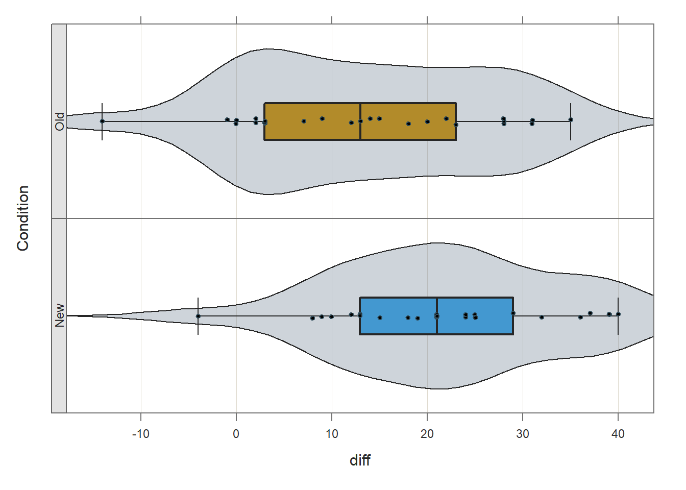
## diff
##   - by levels of -
## Condition
##
##        n   miss     mean       sd      min      mdn      max
## New   25      0    22.04    11.24    -4.00    21.00    40.00
## Old   25      0    13.28    12.79   -14.00    13.00    35.00
##
##        Max Dupli-
## Level   cations   Values
## ------------------------------
## New         3     21 25
## Old         3     3 28
##
## Parameter values (can be manually set)
## -------------------------------------------------------
## size: 0.58      size of plotted points
## out_size: 0.81  size of plotted outlier points
## jitter_y: 1.00 random vertical movement of points
## jitter_x: 0.24  random horizontal movement of points
## bw: 5.23       set bandwidth higher for smoother edges
Based on the violin-box-scatter (VBS) plot depicted in the output from the Plot function, note that (at least visually) the distributions both seem to be roughly normal, and the the variances seem to be roughly equal. These are by no means stringent tests of the statistical assumptions, but they provide us with a cursory understanding of the shape of the distributions and the variances for each of the conditions.
34.2.4.3 Estimate an Independent-Samples t-test with Difference Score Outcome Variable
Now we’re ready to plug the difference score variable (diff) into an independent-samples t-test model as the outcome variable. The between-subjects factor that categorizes trainees based on which condition (Condition) they participated in (New, Old) serves as the predictor variable. As we did above, we will use the ttest function from lessR. To begin, type the name of the ttest function. As the first argument in the parentheses, specify the statistical model. To do so, type the name of the outcome variable (diff) to the left of the ~ operator and the name of the predictor variable (Condition) to the right of the ~ operator. For the second argument, use data= to specify the name of the data frame where the outcome and predictor variables are located (df). For the third argument, type paired=FALSE to inform the function that the data are not paired (i.e., you are not requesting a paired-samples t-test).
# Test of the implied interaction between condition and test time
# Independent-samples t-test with difference score as outcome variable
ttest(diff ~ Condition, # model
      data=df,          # data frame object
      paired=FALSE)     # request independent-samples t-test
##
## Compare diff across Condition with levels New and Old
## Response Variable: diff, diff
## Grouping Variable: Condition,
##
##
## ------ Describe ------
##
## diff for Condition New: n.miss = 0, n = 25, mean = 22.040, sd = 11.238
## diff for Condition Old: n.miss = 0, n = 25, mean = 13.280, sd = 12.785
##
## Mean Difference of diff: 8.760
##
## Weighted Average Standard Deviation: 12.036
##
##
## ------ Assumptions ------
##
## Note: These hypothesis tests can perform poorly, and the
## t-test is typically robust to violations of assumptions.
## Use as heuristic guides instead of interpreting literally.
##
## Null hypothesis, for each group, is a normal distribution of diff.
## Group New Shapiro-Wilk normality test: W = 0.964, p-value = 0.502
## Group Old Shapiro-Wilk normality test: W = 0.954, p-value = 0.309
##
## Null hypothesis is equal variances of diff, homogeneous.
## Variance Ratio test: F = 163.460/126.290 = 1.294, df = 24;24, p-value = 0.532
## Levene's test, Brown-Forsythe: t = -0.983, df = 48, p-value = 0.331
##
##
## ------ Infer ------
##
## --- Assume equal population variances of diff for each Condition
##
## t-cutoff for 95% range of variation: tcut = 2.011
## Standard Error of Mean Difference: SE = 3.404
##
## Hypothesis Test of 0 Mean Diff: t-value = 2.573, df = 48, p-value = 0.013
##
## Margin of Error for 95% Confidence Level: 6.845
## 95% Confidence Interval for Mean Difference: 1.915 to 15.605
##
##
## --- Do not assume equal population variances of diff for each Condition
##
## t-cutoff: tcut = 2.011
## Standard Error of Mean Difference: SE = 3.404
##
## Hypothesis Test of 0 Mean Diff: t = 2.573, df = 47.223, p-value = 0.013
##
## Margin of Error for 95% Confidence Level: 6.848
## 95% Confidence Interval for Mean Difference: 1.912 to 15.608
##
##
## ------ Effect Size ------
##
## --- Assume equal population variances of diff for each Condition
##
## Standardized Mean Difference of diff, Cohen's d: 0.728
##
##
## ------ Practical Importance ------
##
## Minimum Mean Difference of practical importance: mmd
## Minimum Standardized Mean Difference of practical importance: msmd
## Neither value specified, so no analysis
##
##
## ------ Graphics Smoothing Parameter ------
##
## Density bandwidth for Condition New: 6.726
## Density bandwidth for Condition Old: 7.655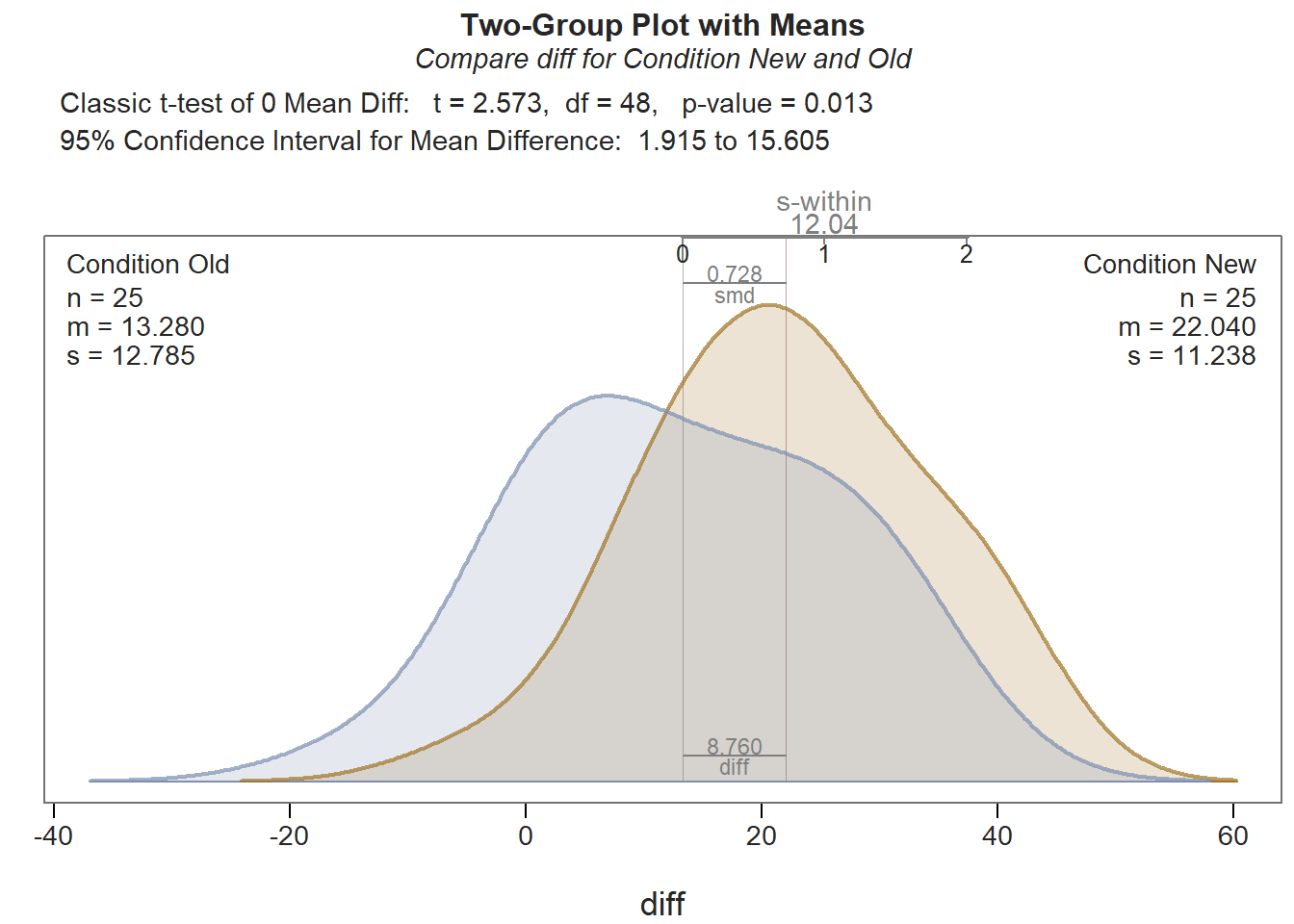
As you can see in the output, the tests of normality (Shapiro-Wilk normality test) and equal variances (Levene’s test) that appear in the Assumptions section indicate that, statistically, there are not significant departures from normality, and there is not evidence of unequal variances. For more information on these tests, please see the earlier chapter on independent-samples t-tests. In the Inference section of the output, the results of the independent-samples t-test (t = 2.573, df = 48, p = .013) indicate that there is evidence that the mean difference scores differ between conditions, as evidence by a p-value that is less than our conventional two-tailed alpha cutoff of .05. Thus, we reject the null hypothesis and conclude that the two means are different from one another. A look at the Description section tells us that the average difference (PostTest minus PreTest) for those who participated in the New training condition is 22.04, and the average difference for those who participated in the Old training condition is 13.28. When considered in tandem with the significant t-test, this indicates that trainees who participated in the new training program showed significantly greater increases in their assessment scores from before to after training than those trainees who participated in the old training program. Essentially, we are interpreting what would be a significant interaction from a statistically equivalent 2x2 mixed-factorial ANOVA model. Because we found a statistically significant difference in means, let’s interpret the effect size (Cohen’s d) as an indicator of practical significance. In the output, d is equal to .73, which is considered to be a medium-large effect, according to conventional rules-of-thumb (see table below). Please note that typically we only interpret practical significance when a difference between means is statistically significant.
| Cohen’s d | Description |
|---|---|
| \(\ge .20\) | Small |
| \(\ge .50\) | Medium |
| \(\ge .80\) | Large |
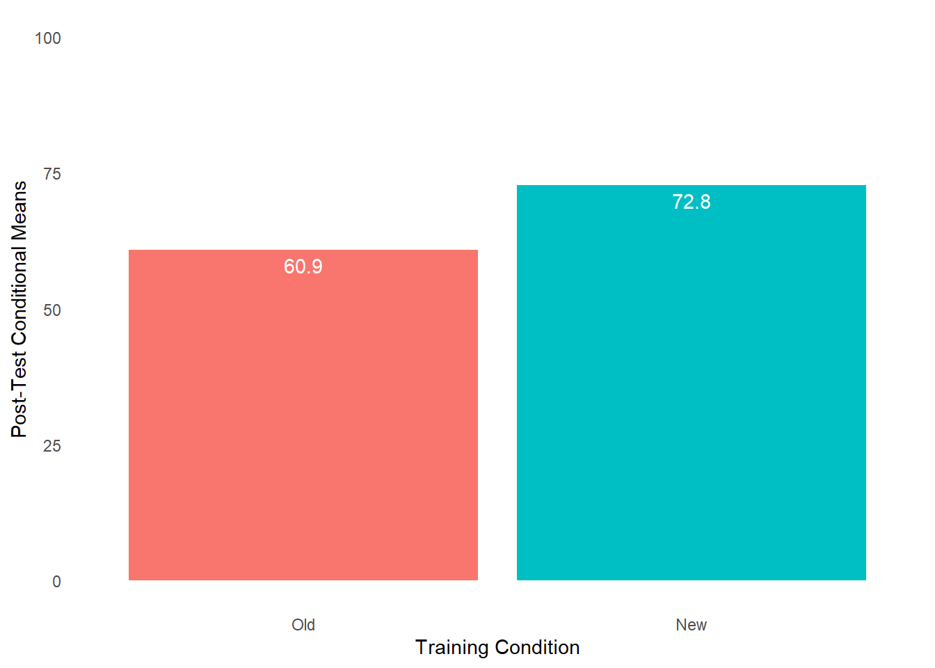
When we find a statistically significant difference between two means based on an independent-samples t-test, it is customary to present the two means in a bar chart. We will use the BarChart function from lessR to do so.
To begin, type the name of the BarChart function. As the first argument, specify x= followed by the name of the categorical (nominal, ordinal) predictor variable, which in this example is Condition. As the second argument, specify y= followed by the name of the continuous (interval, ratio) outcome variable, which in this example is diff. As the third, argument specify stat="mean" to request that the mean of the y= variable be computed by levels of the x= variable. As the fourth argument, specify data= followed by the name of the data frame object (df) to which the x= and y= variables belong. As the fifth argument, use the xlab= to provide a new x-axis label, which for our example will be “Training Condition”. As the sixth argument, use the ylab= to provide a new y-axis label, which for our example will be “Average Difference Score”.
# Create bar chart
BarChart(x=Condition,                     # categorical predictor variable
         y=diff,                          # continuous outcome variable
         stat="mean",                     # request computation of means
         data=df,                         # data frame object
         xlab="Training Condition",       # x-axis label
         ylab="Average Difference Score") # y-axis label
## diff
## - by levels of -
## Condition
##
## n miss mean sd min mdn max
## New 25 0 22.04 11.24 -4.00 21.00 40.00
## Old 25 0 13.28 12.79 -14.00 13.00 35.00
## >>> Suggestions
## Plot(diff, Condition) # lollipop plot
##
##  Plotted Values
##  --------------
##      New     Old
##   22.040  13.280
As noted above, our statistically significant finding from the independent-samples t-test with difference score outcome variable is the equivalent of finding a statistically significant interaction term as part of a 2x2 mixed-factorial ANOVA model. Specifically, our finding implies a statistically significant interaction term between the between-subjects Condition variable and within-subjects Test variable. When a significant interaction is found, it is customary to investigate the simple effects. Given our 2x2 design, our job examining the simple effects is made easier. Next up, we’ll begin with the evaluating the between-subjects simple effects.
34.2.4.4 Evaluate the Between-Subjects Simple Effects
Given that our data are from 2x2 mixed-factorial design, we have two between-subjects simple effects to evaluate: (a) difference between the New and Old conditions’ PreTest means, and (b) difference between the New and Old conditions’ PostTest means. We’ll begin with the evaluating whether there is a difference between the training and control conditions’ PreTest means.
In general, when pre-test data are available, it’s a good idea to determine whether the training and control conditions have different means on the pre-test (PreTest) variable, which were collected prior to individuals’ participation in their respective training conditions. Ideally, our hope is that the average pre-test scores can be treated as equivalent, as this would indicate that the trainees started at about the same place prior to training, suggesting that they are perhaps equivalent groups.
Before applying the ttest function lessR, we will use the Plot function from lessR to visually inspect the distribution of the PreTest variable in each level of the Condition variable. To do so, type the name of the Plot function. As the first argument within the function, type the name of the continuous variable of interest (PreTest). As the second argument, type data= followed by the name of the data frame (df). As the third argument, type by1= followed by the name of the grouping variable (Condition), as this will create the trellis/lattice structure wherein two VBS plots will be created (one for each condition/group).
# VBS plots of the PreTest distributions by Condition
Plot(PreTest,       # outcome variable
     data=df,       # data frame object
     by1=Condition) # grouping variable
## [Trellis graphics from Deepayan Sarkar's lattice package]
##
## >>> Suggestions
## Plot(PreTest, out_cut=2, fences=TRUE, vbs_mean=TRUE) # Label two outliers ...
## Plot(PreTest, box_adj=TRUE) # Adjust boxplot whiskers for asymmetry
## ttest(PreTest ~ Condition) # Add the data parameter if not the d data frame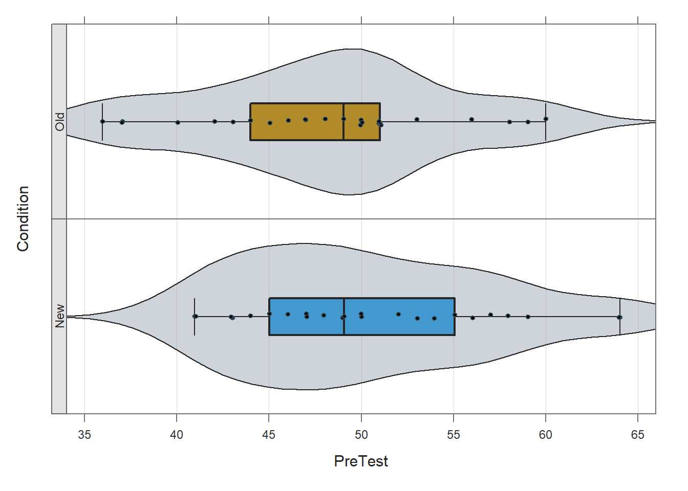
## PreTest
##   - by levels of -
## Condition
##
##        n   miss     mean       sd      min      mdn      max
## New   25      0    50.32     6.72    41.00    49.00    64.00
## Old   25      0    48.04     6.60    36.00    49.00    60.00
##
##        Max Dupli-
## Level   cations   Values
## ------------------------------
## New         3     43
## Old         4     51
##
## Parameter values (can be manually set)
## -------------------------------------------------------
## size: 0.55      size of plotted points
## out_size: 0.80  size of plotted outlier points
## jitter_y: 1.00 random vertical movement of points
## jitter_x: 0.28  random horizontal movement of points
## bw: 2.69       set bandwidth higher for smoother edges
Based on the violin-box-scatter (VBS) plot depicted in the output from the Plot function, note that (at least visually) the distributions both seem to be roughly normally, and the the variances seem to be roughly equal.
Like before, we will estimate this independent-samples t-test using the ttest function from the lessR package. In this model, however, we include the PreTest variable as the outcome variable in our model, but other than that, the arguments will remain the same as our arguments for the previous independent-samples t-test involving the difference variable (diff).
# Between-subjects simple effect:
# Independent-samples t-test with PreTest as outcome variable
ttest(PreTest ~ Condition, # model
      data=df,             # data frame object
      paired=FALSE)        # request independent-samples t-test
##
## Compare PreTest across Condition with levels New and Old
## Response Variable: PreTest, PreTest
## Grouping Variable: Condition,
##
##
## ------ Describe ------
##
## PreTest for Condition New: n.miss = 0, n = 25, mean = 50.320, sd = 6.719
## PreTest for Condition Old: n.miss = 0, n = 25, mean = 48.040, sd = 6.598
##
## Mean Difference of PreTest: 2.280
##
## Weighted Average Standard Deviation: 6.659
##
##
## ------ Assumptions ------
##
## Note: These hypothesis tests can perform poorly, and the
## t-test is typically robust to violations of assumptions.
## Use as heuristic guides instead of interpreting literally.
##
## Null hypothesis, for each group, is a normal distribution of PreTest.
## Group New Shapiro-Wilk normality test: W = 0.947, p-value = 0.220
## Group Old Shapiro-Wilk normality test: W = 0.965, p-value = 0.521
##
## Null hypothesis is equal variances of PreTest, homogeneous.
## Variance Ratio test: F = 45.143/43.540 = 1.037, df = 24;24, p-value = 0.930
## Levene's test, Brown-Forsythe: t = 0.241, df = 48, p-value = 0.811
##
##
## ------ Infer ------
##
## --- Assume equal population variances of PreTest for each Condition
##
## t-cutoff for 95% range of variation: tcut = 2.011
## Standard Error of Mean Difference: SE = 1.883
##
## Hypothesis Test of 0 Mean Diff: t-value = 1.211, df = 48, p-value = 0.232
##
## Margin of Error for 95% Confidence Level: 3.787
## 95% Confidence Interval for Mean Difference: -1.507 to 6.067
##
##
## --- Do not assume equal population variances of PreTest for each Condition
##
## t-cutoff: tcut = 2.011
## Standard Error of Mean Difference: SE = 1.883
##
## Hypothesis Test of 0 Mean Diff: t = 1.211, df = 47.984, p-value = 0.232
##
## Margin of Error for 95% Confidence Level: 3.787
## 95% Confidence Interval for Mean Difference: -1.507 to 6.067
##
##
## ------ Effect Size ------
##
## --- Assume equal population variances of PreTest for each Condition
##
## Standardized Mean Difference of PreTest, Cohen's d: 0.342
##
##
## ------ Practical Importance ------
##
## Minimum Mean Difference of practical importance: mmd
## Minimum Standardized Mean Difference of practical importance: msmd
## Neither value specified, so no analysis
##
##
## ------ Graphics Smoothing Parameter ------
##
## Density bandwidth for Condition New: 4.012
## Density bandwidth for Condition Old: 3.950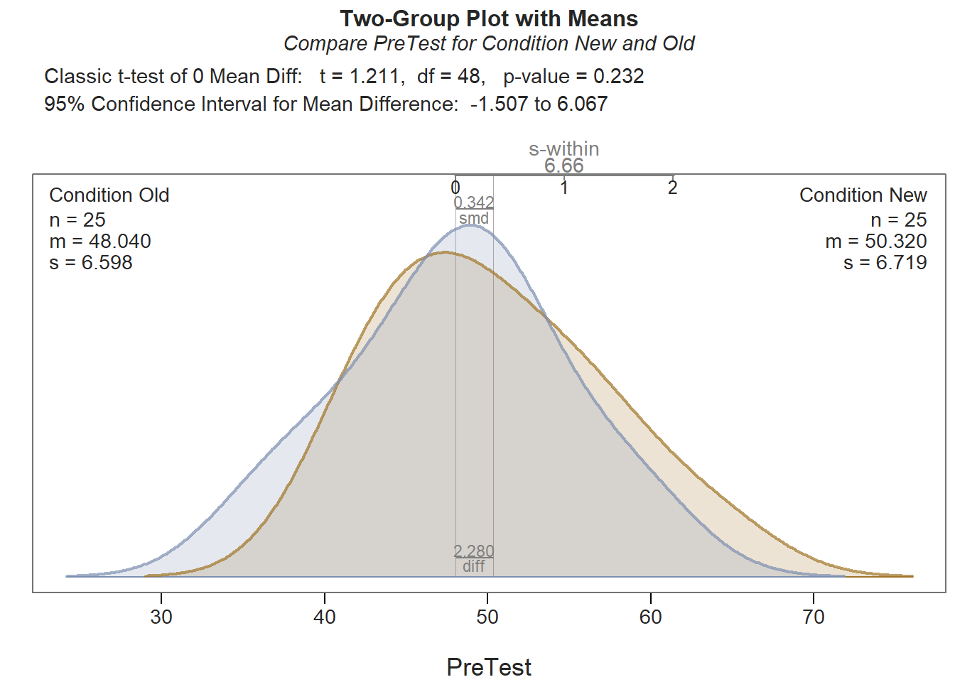
As you can see in the output, the tests of normality (Shapiro-Wilk normality test) and equal variances (Levene’s test) indicate that, statistically, there are neither significant departures from normality nor evidence of unequal variances. The results of the independent-samples t-test itself (t = 1.211, df = 48, p = .232) indicate that there is no evidence that the mean pre-test scores differ between conditions, as evidenced by a p-value that is equal to or greater than our conventional two-tailed alpha cutoff of .05. Thus, we fail to reject the null hypothesis and conclude that the two means equal. This finding suggests that the New and Old conditions were roughly equivalent in terms of PreTest scores prior to engaging in training.
Next, we will evaluate whether the means on the PostTest variable differ significantly between the New and Old conditions. Before doing so, we will once again use the Plot function from lessR to visually inspect the distribution of the PostTest variable in each level of the Condition variable. To do so, type the name of the Plot function. As the first argument within the function, type the name of the continuous variable of interest (PostTest). As the second argument, type data= followed by the name of the data frame (df). As the third argument, type by1= followed by the name of the grouping variable (Condition), as this will create the trellis/lattice structure wherein two VBS plots will be created (one for each condition/group).
# VBS plots of the PostTest distributions by Condition
Plot(PostTest,      # outcome variable
     data=df,       # data frame object
     by1=Condition) # grouping variable
## [Trellis graphics from Deepayan Sarkar's lattice package]
##
## >>> Suggestions
## Plot(PostTest, out_cut=2, fences=TRUE, vbs_mean=TRUE) # Label two outliers ...
## Plot(PostTest, box_adj=TRUE) # Adjust boxplot whiskers for asymmetry
## ttest(PostTest ~ Condition) # Add the data parameter if not the d data frame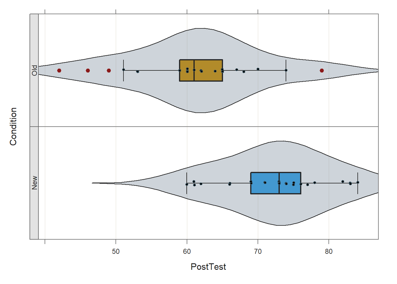
## PostTest
##   - by levels of -
## Condition
##
##        n   miss     mean       sd      min      mdn      max
## New   25      0    72.36     6.98    60.00    73.00    84.00
## Old   25      0    61.32     9.15    42.00    61.00    79.00
##
##        Max Dupli-
## Level   cations   Values
## ------------------------------
## New         4     73
## Old         4     60
##
## Parameter values (can be manually set)
## -------------------------------------------------------
## size: 0.55      size of plotted points
## out_size: 0.80  size of plotted outlier points
## jitter_y: 1.00 random vertical movement of points
## jitter_x: 0.28  random horizontal movement of points
## bw: 4.43       set bandwidth higher for smoother edges
The two violin-box-scatter (VBS) plots visually suggest that the distributions are roughly normal and the varainces are roughly equal.
Now we are ready to apply an independent-samples t-test, except this time, we will specify the PostTest variable as the outcome variable.
# Between-subjects simple effect:
# Independent-samples t-test with PostTest as outcome variable
ttest(PostTest ~ Condition, # model
      data=df,              # data frame object
      paired=FALSE)         # request independent-samples t-test
##
## Compare PostTest across Condition with levels New and Old
## Response Variable: PostTest, PostTest
## Grouping Variable: Condition,
##
##
## ------ Describe ------
##
## PostTest for Condition New: n.miss = 0, n = 25, mean = 72.360, sd = 6.975
## PostTest for Condition Old: n.miss = 0, n = 25, mean = 61.320, sd = 9.150
##
## Mean Difference of PostTest: 11.040
##
## Weighted Average Standard Deviation: 8.136
##
##
## ------ Assumptions ------
##
## Note: These hypothesis tests can perform poorly, and the
## t-test is typically robust to violations of assumptions.
## Use as heuristic guides instead of interpreting literally.
##
## Null hypothesis, for each group, is a normal distribution of PostTest.
## Group New Shapiro-Wilk normality test: W = 0.950, p-value = 0.253
## Group Old Shapiro-Wilk normality test: W = 0.969, p-value = 0.621
##
## Null hypothesis is equal variances of PostTest, homogeneous.
## Variance Ratio test: F = 83.727/48.657 = 1.721, df = 24;24, p-value = 0.191
## Levene's test, Brown-Forsythe: t = -0.955, df = 48, p-value = 0.344
##
##
## ------ Infer ------
##
## --- Assume equal population variances of PostTest for each Condition
##
## t-cutoff for 95% range of variation: tcut = 2.011
## Standard Error of Mean Difference: SE = 2.301
##
## Hypothesis Test of 0 Mean Diff: t-value = 4.798, df = 48, p-value = 0.000
##
## Margin of Error for 95% Confidence Level: 4.627
## 95% Confidence Interval for Mean Difference: 6.413 to 15.667
##
##
## --- Do not assume equal population variances of PostTest for each Condition
##
## t-cutoff: tcut = 2.014
## Standard Error of Mean Difference: SE = 2.301
##
## Hypothesis Test of 0 Mean Diff: t = 4.798, df = 44.852, p-value = 0.000
##
## Margin of Error for 95% Confidence Level: 4.635
## 95% Confidence Interval for Mean Difference: 6.405 to 15.675
##
##
## ------ Effect Size ------
##
## --- Assume equal population variances of PostTest for each Condition
##
## Standardized Mean Difference of PostTest, Cohen's d: 1.357
##
##
## ------ Practical Importance ------
##
## Minimum Mean Difference of practical importance: mmd
## Minimum Standardized Mean Difference of practical importance: msmd
## Neither value specified, so no analysis
##
##
## ------ Graphics Smoothing Parameter ------
##
## Density bandwidth for Condition New: 4.175
## Density bandwidth for Condition Old: 5.464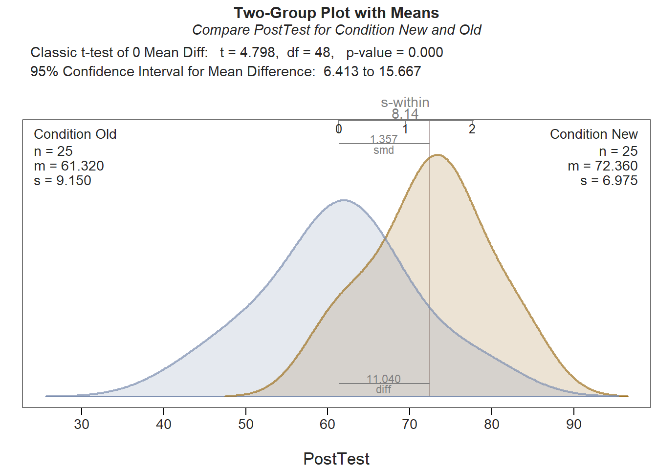
We find that the scores on the PostTest are statistically significant higher for those in the New training condition (72.360) than those in the Old training condition (64.320) (t = 4.798, df = 48, p < .001), and this effect is very large (Cohen’s d = 1.357).
In sum, the between-subjects simple effects help us understand the nature of the implied interaction we observed in our focal independent-samples t-test with difference score outcome variable. Putting everything together to this point, we have found that individuals started in approximately the same place in terms of pre-test scores prior to participating in their respective training programs, those who participated in the New training program showed, on average, a greater increase in scores from pre-test to post-test than those who participated in the Old training program, and those who participated in the New training program showed, on average, higher post-test scores than those who participated in the Old training program.
34.2.4.5 Evaluate the Within-Subjects Simple Effects
To compute the within-subjects simple effects, we will apply paired-samples t-tests to each level of the between-subjects factor (Condition). To do so, we will use the ttest function from lessR once more. For more information about a paired-samples t-test, please check the earlier chapter.
Let’s begin by evaluating whether the mean of the differences resulting from the PreTest and PostTest variables differs significantly from zero for those individuals who participated in the New training condition. In this context, we can think of our PreTest variable as representing the first level of within-subjects variable representing test time, and the PostTest variable as representing the second level of within-subjects variable representing test time. As the first argument in the ttest function, specify the PreTest variable. As the second argument, specify the PostTest variable. As the third argument, specify data= followed by the name of data frame object (df). As the fourth argument, specify paired=TRUE to request an paired-samples t-test. As the fifth argument, specify rows=(Condition=="New") to filter the data frame down to just those individuals who participated in the New training condition.
# Within-subjects simple effect:
# Paired-samples t-test for just New training condition
ttest(PreTest,                 # first level of within-subjects variable
      PostTest,                # second level of within-subjects variable
      data=df,                 # data frame object
      paired=TRUE,             # paired-samples t-test
      rows=(Condition=="New")) # first level of between-subjects variable
##
##
## ------ Describe ------
##
## Difference: n.miss = 0, n = 25, mean = 22.040, sd = 11.238
##
##
## ------ Normality Assumption ------
##
## Null hypothesis is a normal distribution of Difference.
## Shapiro-Wilk normality test: W = 0.9641, p-value = 0.502
##
##
## ------ Infer ------
##
## t-cutoff for 95% range of variation: tcut = 2.064
## Standard Error of Mean: SE = 2.248
##
## Hypothesized Value H0: mu = 0
## Hypothesis Test of Mean: t-value = 9.806, df = 24, p-value = 0.000
##
## Margin of Error for 95% Confidence Level: 4.639
## 95% Confidence Interval for Mean: 17.401 to 26.679
##
##
## ------ Effect Size ------
##
## Distance of sample mean from hypothesized: 22.040
## Standardized Distance, Cohen's d: 1.961
##
##
## ------ Graphics Smoothing Parameter ------
##
## Density bandwidth for 6.726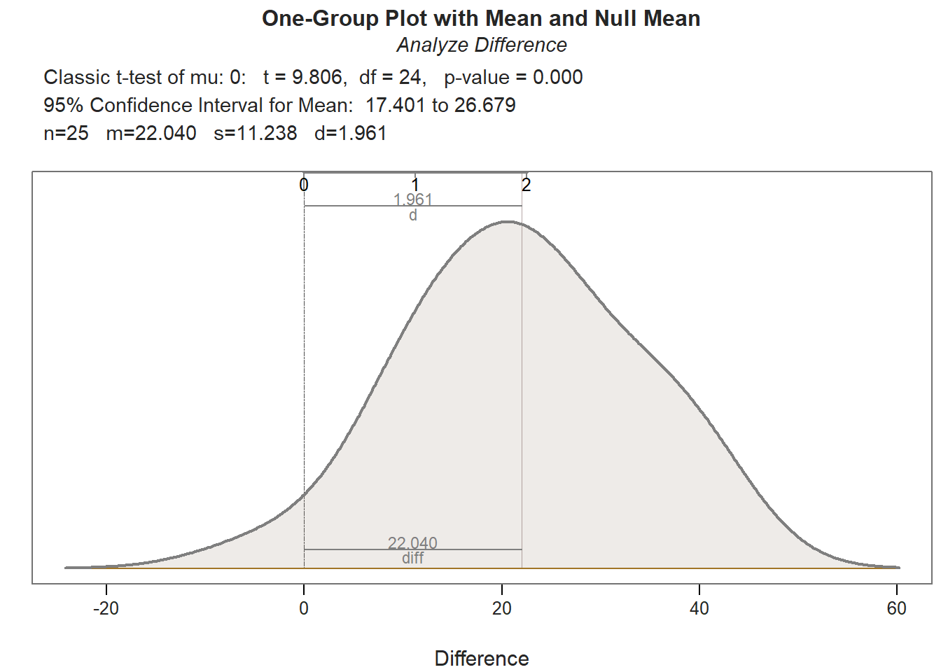
Let’s repeat the process for the those individuals who participated in the Old training condition.
# Within-subjects simple effect:
# Paired-samples t-test for just Old training condition
ttest(PreTest,                 # first level of within-subjects variable
      PostTest,                # second level of within-subjects variable
      data=df,                 # data frame object
      paired=TRUE,             # paired-samples t-test
      rows=(Condition=="Old")) # second level of between-subjects variable
##
##
## ------ Describe ------
##
## Difference: n.miss = 0, n = 25, mean = 13.280, sd = 12.785
##
##
## ------ Normality Assumption ------
##
## Null hypothesis is a normal distribution of Difference.
## Shapiro-Wilk normality test: W = 0.9541, p-value = 0.309
##
##
## ------ Infer ------
##
## t-cutoff for 95% range of variation: tcut = 2.064
## Standard Error of Mean: SE = 2.557
##
## Hypothesized Value H0: mu = 0
## Hypothesis Test of Mean: t-value = 5.194, df = 24, p-value = 0.000
##
## Margin of Error for 95% Confidence Level: 5.277
## 95% Confidence Interval for Mean: 8.003 to 18.557
##
##
## ------ Effect Size ------
##
## Distance of sample mean from hypothesized: 13.280
## Standardized Distance, Cohen's d: 1.039
##
##
## ------ Graphics Smoothing Parameter ------
##
## Density bandwidth for 7.655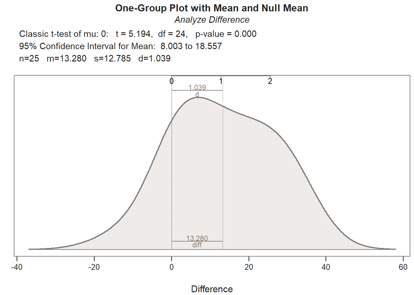
Both paired-samples t-tests met the normality assumption. Further, the within-subjects simple effects gleaned from these paired-samples t-tests showed a statistically significant mean of the differences (PostTest minus PreTest); however, the mean of the differences for those who participated in the New training condition (Mean of the Differences = 22.040, t = 9.806, df = 24, p < .001, Cohen’s d = 1.961) was notably larger than the mean of the differences for those who participated in the Old training condition (Mean of the Differences = 13.280, t = 5.194, df = 24, p < .001, Cohen’s d = 1.039). This further elucidates what we observed in our initial independent-samples t-test in which the difference score variable served as the outcome; specifically, we now know that the average increase in test scores for those in the New training program is statistically significantly different from zero and very large, whereas the average increase in test scores for those in the Old training program is statistically significant and large – but not nearly as large in a relative sense.
Together, the between-subjects and within-subjects simple effects help us understand the nature of the implied interaction we observed in our focal independent-samples t-test with difference score outcome variable. In sum, we found: (a) Individuals started in approximately the same place in terms of pre-test scores prior to participating in their respective training programs; (b) Those who participated in the New training program showed, on average, a greater increase in scores from pre-test to post-test than those who participated in the Old training program; more specifically, those who participated in both the New and Old training programs showed large increases in test scores, with those in the New training programs showing what can be described as a much larger increase; (c) Those who participated in the New training program showed, on average, higher post-test scores than those who participated in the Old training program, which indicates that those in the New training program ended up with higher post-test scores.
34.2.5 Summary
In this chapter, we learned how to estimate an independent-samples t-test with a difference score outcome variable to evaluate a 2x2 mixed-factorial design like a pre-test/post-test with control group design; importantly, this approach is statistically equivalent to a 2x2 mixed-factorial ANOVA when there is a balanced design. We also learned how to estimate the between-subjects and within-subjects simple effects.
34.3 Chapter Supplement
In this chapter supplement, we will learn how, under these conditions, a simple linear regression model with difference score outcome variable, biserial correlation with difference score outcome variable, 2x2 mixed-factorial ANOVA model, and random-coefficients model will yield results that are statistically equivalent to the independent-samples t-test with difference score outcome variable that was introduced in the main portion of this chapter. And at the very end of the chapter, we will learn how to estimate an analysis of covariance (ANCOVA) model, which is not statistically equivalent to the aforementioned approaches, but, in spite of a less intuitive interpretation typically offers greater statistical power and estimation precision (Bodner and Bliese 2018).
34.3.1 Functions & Packages Introduced
| Function | Package |
|---|---|
factor |
base R |
lm |
base R |
summary |
base R |
as.numeric |
base R |
cor.test |
base R |
pivot_longer |
tidyr |
aov |
base R |
model.tables |
base R |
t.test |
base R |
interaction.plot |
base R |
lme |
nlme |
anova |
base R |
tapply |
base R |
list |
base R |
mean |
base R |
Anova |
car |
glht |
multcomp |
emmeans |
emmeans |
diff |
base R |
34.3.2 Initial Steps
If required, please refer to the Initial Steps section from this chapter for more information on these initial steps.
# Install readr package if you haven't already
# [Note: You don't need to install a package every
# time you wish to access it]
install.packages("readr")
# Access readr package
library(readr)
# Read data and name data frame (tibble) object
df <- read_csv("TrainingEvaluation_PrePostControl.csv")## Rows: 50 Columns: 4
## ── Column specification ────────────────────────────────────────────────────────────────────────────────────────────────────────────
## Delimiter: ","
## chr (1): Condition
## dbl (3): EmpID, PreTest, PostTest
##
## ℹ Use `spec()` to retrieve the full column specification for this data.
## ℹ Specify the column types or set `show_col_types = FALSE` to quiet this message.## [1] "EmpID" "Condition" "PreTest" "PostTest"## spc_tbl_ [50 × 4] (S3: spec_tbl_df/tbl_df/tbl/data.frame)
## $ EmpID : num [1:50] 26 27 28 29 30 31 32 33 34 35 ...
## $ Condition: chr [1:50] "New" "New" "New" "New" ...
## $ PreTest : num [1:50] 41 56 50 45 41 48 64 46 47 47 ...
## $ PostTest : num [1:50] 66 74 62 84 78 73 60 61 71 83 ...
## - attr(*, "spec")=
## .. cols(
## .. EmpID = col_double(),
## .. Condition = col_character(),
## .. PreTest = col_double(),
## .. PostTest = col_double()
## .. )
## - attr(*, "problems")=<externalptr>## # A tibble: 6 × 4
## EmpID Condition PreTest PostTest
## <dbl> <chr> <dbl> <dbl>
## 1 26 New 41 66
## 2 27 New 56 74
## 3 28 New 50 62
## 4 29 New 45 84
## 5 30 New 41 78
## 6 31 New 48 73As an initial step, we must create a difference score variable. To do so, we must first specify the name of the existing data frame we wish to add this new variable to (df), followed by the $ symbol and what we would like to name this new difference variable; in this example, I name the new variable diff. Second, type the <- symbol to indicate that you are creating and naming a new object. Third, write simple arithmetic equation wherein PreTest scores are subtracted from PostTest scores, which means that a positive difference will indicate an increase in assessment scores from PreTest to PostTest.
34.3.3 Estimating a Simple Linear Regression Model with a Difference Score Outcome Variable
Prior to estimating a simple linear regression model, let’s re-order the default levels of the Condition variable from alphabetical (“New”, “Old”) to “Old” preceding “New”. This will ensure that the sign of the effect is comparable to what we found with the independent-samples t-test with a difference score outcome variable. To do so, we’ll convert the Condition variable to type factor using the factor function from base R. As the first argument, we’ll specify the name of the data frame object from the main portion of the chapter (df) followed by the $ operator and the name of the Condition variable. As the second argument, we’ll specify the levels= argument followed by the c function; as the two arguments within the c function, we’ll specify “Old” as the first argument and “New” as the second argument.
# Re-order Condition variable and convert to a factor
df$Condition <- factor(df$Condition,
                       levels=c("Old", "New"))
To estimate a simple linear regression model, we will use the lm function from base R. We’ll assign the model to an object we name lm_mod using the <- assignment operator. As the first argument in the lm function, we’ll specify our model, which is the diff (difference score variable) regressed on the Condition variable. As the second argument, we’ll specify data= followed by the name of the data frame object to which the variables in the model belong (df). Finally, we will print a summary of the results using the summary function from base R with the name of our model object as the sole parenthetical argument (lm_mod).
# Estimate simple linear regression model
lm_mod <- lm(diff ~ Condition,
             data=df)

# Print a summary of the model results
summary(lm_mod)
##
## Call:
## lm(formula = diff ~ Condition, data = df)
##
## Residuals:
## Min 1Q Median 3Q Max
## -27.28 -10.22 -0.66 9.47 21.72
##
## Coefficients:
## Estimate Std. Error t value Pr(>|t|)
## (Intercept) 13.280 2.407 5.517 0.00000136 ***
## ConditionNew 8.760 3.404 2.573 0.0132 *
## ---
## Signif. codes: 0 '***' 0.001 '**' 0.01 '*' 0.05 '.' 0.1 ' ' 1
##
## Residual standard error: 12.04 on 48 degrees of freedom
## Multiple R-squared: 0.1212, Adjusted R-squared: 0.1029
## F-statistic: 6.621 on 1 and 48 DF, p-value: 0.01322In the output, the unstandardized regression coefficient associated with the Condition variable is 8.760, the standard error is 3.404, the t-value is 2.573, the degrees of freedom (df) is equal to 48, and the p-value is .0132, all of which are equal to the corresponding statistics found using the independent-samples t-test. In fact, the coefficient value of 8.760 is the mean difference between the two “Old” and “New” conditions that we observed in the independent-samples t-test with a difference score outcome variable. Finally, please note that unadjusted R-squared (R2) for the model is .1212, which we will revisit in the context of the biserial correlation in the following section.
34.3.4 Estimating a Biserial Correlation with a Difference Score Outcome Variable
Under these conditions, a biserial correlation is also statistically equivalent to an independent-samples t-test with a difference score outcome variable. Before we estimate the biserial correlation, however, we need to convert the Condition variable to type numeric, as the correlation function we will use expects numeric variables. To do so, we will use the as.numeric function from base R. Let’s name this converted variable Condition_numeric and attach it to our df data frame object using the $ operator. The <- assignment operator will allow us to perform this assignment. To the right of the <- assignment operator, let’s type the name of the as.numeric function, and as the sole parenthetical argument, we will specify the data frame df followed by the $ operator and the Condition variable.
# Convert Condition variable to numeric and assign to new variable
df$Condition_numeric <- as.numeric(df$Condition)
We will estimate the biserial correlation using the cor.test function base R. As the first argument, we’ll specify the data frame df followed by the $ operator and the Condition_numeric variable. As the second argument, we’ll specify the data frame df followed by the $ operator and the diff (difference score) variable.
##
##  Pearson's product-moment correlation
##
## data:  df$Condition_numeric and df$diff
## t = 2.5731, df = 48, p-value = 0.01322
## alternative hypothesis: true correlation is not equal to 0
## 95 percent confidence interval:
##  0.07730703 0.57115937
## sample estimates:
##       cor
## 0.3481629
Like the independent-samples t-test and simple linear regression model with a difference score outcome variable, the following model statistics are the same for the biserial correlation: t = 2.573, df = 48, and p = .0132. Further, the correlation coefficient is .3481629, and if we square that value, we get an unadjusted R-squared (R2) equal to .1212, which is the same R-squared value as our simple linear regression model. Thus, under these conditions, the biserial correlation is also statistically equivalent to the independent-samples t-test and simple linear regression model with a difference score outcome variable.
Before moving on, let’s remove the Condition_numeric variable from our df data frame object to avoid confusion when we proceed to the following section.
34.3.5 Estimating a 2x2 Mixed-Factorial ANOVA Model
When there is a balanced design, a 2x2 mixed-factorial analysis of variance (ANOVA) model will also be statistically equivalent to a independent-samples t-test, simple linear regression model, and biserial correlation with a difference score outcome variable.
As conceptual background, a 2x2 mixed-factorial ANOVA is a specific application of a factorial analysis of variance (ANOVA), which is itself part of a larger family of analyses aimed at comparing means. A factorial ANOVA is used to compare the means for two or more categorical (nominal, ordinal) predictor (independent) variables (e.g., conditions, populations). The word “factorial” in ANOVA implies that there are two or more factors (i.e., categorical predictor variables). Just like a one-way ANOVA, a factorial ANOVA has a single continuous (interval, ratio) outcome (dependent) variable. A factorial ANOVA with just two factors, is often referred to as a two-way ANOVA, where the “two” refers to two factors. A factorial ANOVA can include within-subjects factors, between-subjects factors, or a combination of the two. When we have at least one within-subjects (e.g., repeated measurements for same cases) factor and at least one between-subjects (e.g., each case assigned to just one level of factor), we commonly refer to this as a mixed-factorial ANOVA.
When we are working with data acquired from a pre-test/post-test with control group and random assignment design, a 2x2 mixed-factorial ANOVA is an example of an appropriate statistical analysis, and in the training context. When we have a mixed-factorial design, we are typically interested in looking at the interaction between the two or more factors (i.e., predictor variables). That is, we want to know if differences in means between levels of one factor is conditional on levels of another factor. For example, in a 2x2 mixed-factorial ANOVA used in training evaluation, we might wish to know whether average change in assessment scores from pre-test to post-test is conditional on the training condition (training vs. control). Presumably, we would hope that the average change in assessment scores from pre-test to post-test is larger in the training condition than the control condition.
In this chapter, we have thus far assumed our data were acquired from a balanced design, which means that the same number of employees participated in the training and control conditions and that each person completed the pre-test and post-test; in other words, there is an equal number of observations in the four cells associated with this 2x2 mixed factorial design. And we will continue to assume that our data are from a balanced design. The reason being, when there is a balanced design, a 2x2 mixed-factorial ANOVA with Type I sum of squares (see below) will be statistically equivalent to an independent-samples t-test in which the continuous (interval, ratio) outcome (dependent) variable represents the difference between the two levels of the within-subjects factor (e.g., post-test minus pre-test) and the predictor (independent) variable is the between-subjects factor (e.g., condition: old training program, new training program).
Type I sum of squares is the default approach to calculating sum of squares in most R ANOVA functions. Type II and Type III sum of squares refer to the other approaches to calculating sum of squares for an ANOVA. Results are typically similar between Type I, Type II, and Type III approaches when the data are balanced across groups designated by the factors (i.e., predictor variables). To apply Type II or Type III sum of squares, I recommend using the Anova function from the car package. If you wish to learn more about Type I, II, and III sum of squares (SS), I recommend checking out this link.
To estimate the 2x2 mixed-factorial ANOVA model, we will use the same data frame object as in the main portion of the chapter, except we will need to perform data manipulation to pivot the data frame from wide to long format, and we will need to convert some of the variables to factors and re-order their levels.
The data frame from the main portion of the chapter (df) is in wide format, as each substantive variable has its own column. To restructure the data from wide to long format, we will use the pivot_longer function from the tidyr package. Along with readr and dplyr (as well as other useful packages), the tidyr package is part of the tidyverse of packages. Let’s begin by installing and accessing the tidyr package so that we can use the pivot_longer function.
Note. If you received an error when attempting to access the tidyr package using the library function, you may need to install the following packages using the install.packages function: rlang and glue. Alternatively, you may try installing the entire tidyverse package.
Now that we’ve accessed the tidyr package, I will demonstrate how to manipulate the data from wide-to-long format using the pipe operator (%>%). The pipe operator comes from a package called magrittr, on which the tidyr package is partially dependent. In short, a pipe allows a person to more efficiently write code and to improve the readability of the code and overall script. Specifically, a pipe forwards the result or value of one object or expression to a subsequent function. In doing so, one can avoid writing functions in which other functions are nested parenthetically. For more information on the pipe operator, check out Wickham and Grolemund’s chapter on pipes.
Using the pipe (%>%) operator technique, let’s apply the pivot_longer function to manipulate the df data frame object from wide format to long format.
We can specify the wide-to-long manipulation as follows.
- Create a name for a new data frame object to which we will eventually assign a long-format data frame object; here, I name the new data frame object
df_long. - Use the
<-operator to assign the new long-form data frame object to the object nameddf_longin the step above. - Type the name of the original data frame object (
df), followed by the pipe (%>%) operator. - Type the name of the
pivot_longerfunction.
- As the first argument in the
pivot_longerfunction, typecols=followed by thec(combine) function. As the arguments within thecfunction, list the names of the variables that you wish to pivot from separate variables (wide) to levels or categories of a new variable, effectively stacking them vertically. In this example, let’s list the names of pre-test and post-test variables:PreTestandPostTest. - As the second argument in the
pivot_longerfunction, typenames_to=followed by what you would like to name the new stacked variable (see previous) created from the four survey measure variables. Let’s call the new variable containing the names of the pre-test and post-test variables the following:"Test". - As the third argument in the
pivot_longerfunction, typevalues_to=followed by what you would like to name the new variable that contains the scores for the two variables that are now stacked vertically for each case. Let’s call the new variable containing the scores on the two variables the following:"Score".
# Apply pivot_longer function to restructure data to long format (using pipe)
df_long <- df %>%
  pivot_longer(cols=c(PreTest, PostTest),
               names_to="Test",
               values_to="Score")

# Print first 12 rows of new data frame
head(df_long, n=12)
## # A tibble: 12 × 5
## EmpID Condition diff Test Score
## <dbl> <fct> <dbl> <chr> <dbl>
## 1 26 New 25 PreTest 41
## 2 26 New 25 PostTest 66
## 3 27 New 18 PreTest 56
## 4 27 New 18 PostTest 74
## 5 28 New 12 PreTest 50
## 6 28 New 12 PostTest 62
## 7 29 New 39 PreTest 45
## 8 29 New 39 PostTest 84
## 9 30 New 37 PreTest 41
## 10 30 New 37 PostTest 78
## 11 31 New 25 PreTest 48
## 12 31 New 25 PostTest 73As you can see, in the output, each employee now has two rows of data – one row for each test measure and the associated score. The giveaway is that each respondent’s unique EmpID value is repeated two times.
Because we no longer need the diff (difference score variable), let’s remove it.
We also need to convert the EmpID variable to type factor. To do so, we’ll use the factor function from base R.
Finally, we will override the default ordering of the “PostTest” and “PreTest” levels of the Test variable from alphabetical to “PreTest” preceding “PostTest”. In doing so, we will also convert the Test variable to type factor using the factor function from base R. We will also override the default ordering of the Condition variable’s from alphabetical to “Old” preceding “New”.
# Re-order Test variable and convert to a factor
df_long$Test <- factor(df_long$Test,
                       levels=c("PreTest", "PostTest"))

# Re-order Condition variable and convert to a factor
df_long$Condition <- factor(df_long$Condition,
                            levels=c("Old", "New"))
We will use the aov function from base R to estimate our ANOVA. Specifically, we will estimate a 2x2 mixed-factorial ANOVA because there is a within-subjects variable (Test) with two levels (“PreTest”, “PostTest”) and a between-subjects variable (Condition) with two levels (“Old”, “New”). We will begin by creating a model object name of our choosing (aov_mod), and we will use the <- assignment operator to assign our fitted model to the object. To the right of the <- assignment operator, we will type the name of the aov function. As the first argument in the function, we will specify the name of our outcome variable (Score) followed by the ~ operator, and to the right of the ~ operator, we will specify the name of our between-subjects variable (Condition) followed by the * interaction operator and then the name of the within-subjects variable (Test); after the within-subjects variable, we will type the + operator followed by the Error function. Within the Error function parentheses, we specify the name of the grouping variable (EmpID, which is the unique employee identifier), followed by a forward slash / and the name of the within-subjects variable (Test); More specifically, the Error function indicates that there is nonindependence in the data, such that we have repeated measures of the Test variable levels nested within employees. As the second argument in the aov function, we will specify the data= argument followed by the name of our long-format df_long data frame object, to which all of the variables specified in our model belong. Finally, we will print the model results using the summary function from base R with the name of the fitted model object in the parentheses (aov_mod).
# Estimate 2x2 mixed factorial ANOVA model
aov_mod <- aov(Score ~               # outcome variable
                 Condition*Test +    # within- & between-subjects interaction
                 Error(EmpID/Test),  # nesting of within-subjects variable
               data=df_long)         # data frame object

# Print a summary of the results
summary(aov_mod)
##
## Error: EmpID
## Df Sum Sq Mean Sq F value Pr(>F)
## Condition 1 1109 1108.9 29.11 0.00000207 ***
## Residuals 48 1829 38.1
## ---
## Signif. codes: 0 '***' 0.001 '**' 0.01 '*' 0.05 '.' 0.1 ' ' 1
##
## Error: EmpID:Test
## Df Sum Sq Mean Sq F value Pr(>F)
## Test 1 7797 7797 107.636 0.0000000000000749 ***
## Condition:Test 1 480 480 6.621 0.0132 *
## Residuals 48 3477 72
## ---
## Signif. codes: 0 '***' 0.001 '**' 0.01 '*' 0.05 '.' 0.1 ' ' 1For the 2x2 mixed-factorial ANOVA model, the interaction term involving the between-subjects Condition variable and within-subjects Test variable produces the following key statistics: F = 6.621 and p = .0132. If we compute the square root of the F-value (6.621), we get 2.573, which is the same as the t-value we observed in the independent-samples t-test, simple linear regression model, and biserial correlation with a difference score outcome variable; plus, the associated p-value (.0132) and the residuals degrees of freedom (48) are also the same.
We can apply the model.tables function from base R with the fitted model object (aov_mod) and “means” as the two function arguments. Doing so provides us with tables of means.
## Tables of means
## Grand mean
##
## 58.01
##
##  Condition
## Condition
##   Old   New
## 54.68 61.34
##
##  Test
## Test
##  PreTest PostTest
##    49.18    66.84
##
##  Condition:Test
##          Test
## Condition PreTest PostTest
##       Old 48.04   61.32
##       New 50.32   72.36
Given the statistically significant interaction term between the between-subjects Condition variable and within-subjects Test variable, we proceed forward with follow-up analyses of the between-subjects and within-subjects simple effects. Given our 2x2 design, our job examining the simple effects is made easier. Let’s begin with the between-subjects simple effects.
To compute the between-subjects simple effects, we will apply independent-samples t-tests to each level of the within-subjects factor. To do so, we will use the t.test function from base R.
- As the first argument, we’ll specify our model, which is our outcome variable (
Score) followed by the~operator and the predictor variable (Condition). - As the second argument, we’ll specify
data=followed by the name of our long-format data frame object (df_long). - As the third argument, we’ll specify
paired=FALSEto request an independent-samples t-test. - As the fourth argument, we’ll assume the variances are equal by applying
var.equal=TRUE. As the fifth argument, we’ll specifysubset=(Test=="PreTest")to filter the data down to just the “PreTest” scores. - We’ll then repeat the prior steps for the
PostTestscores in a separatet.testfunction.
# Between-subjects simple effects for the Condition variable
# by each level of the Test variable

# By PreTest level of Test variable
t.test(Score ~ Condition,
       data=df_long,
       paired=FALSE,
       var.equal=TRUE,
       subset=(Test=="PreTest"))
##
## Two Sample t-test
##
## data: Score by Condition
## t = -1.2106, df = 48, p-value = 0.232
## alternative hypothesis: true difference in means between group Old and group New is not equal to 0
## 95 percent confidence interval:
## -6.066903 1.506903
## sample estimates:
## mean in group Old mean in group New
## 48.04 50.32# By PostTest level of Test variable
t.test(Score ~ Condition,
data=df_long,
paired=FALSE,
var.equal=TRUE,
subset=(Test=="PostTest"))##
## Two Sample t-test
##
## data: Score by Condition
## t = -4.7976, df = 48, p-value = 0.000016
## alternative hypothesis: true difference in means between group Old and group New is not equal to 0
## 95 percent confidence interval:
## -15.666791 -6.413209
## sample estimates:
## mean in group Old mean in group New
## 61.32 72.36For the independent-samples t-test involving just the “PreTest” scores, we find that there is not a statistically significant difference for scores on the “PreTest” between the “New” and “Old” levels of the Condition variable (t = -1.2106, df = 48, p = .232). This tells us that those in the “New” and “Old” training conditions started at about the same place in terms of the scores prior to the training intervention.
For the independent-samples t-test involving just the “PostTest” scores, we find that there is a statistically significant difference for scores on the “PostTest” between the “New” and “Old” levels of the Condition variable (t = -4.7976, df = 48, p < .001). Examining the means informs us that those in the “New” training condition had statistically significantly higher scores on the “PostTest” than those in the “Old” training condition.
To compute the within-subjects simple effects, we will apply paired-samples t-tests to each level of the between-subjects fact. To do so, we will use the t.test function from base R once more.
- As the first argument, we’ll specify our model, which is our outcome variable (
Score) followed by the~operator and the predictor variable (Test). - As the second argument, we’ll specify
data=followed by the name of our long-format data frame object (df_long). - As the third argument, we’ll specify
paired=TRUEto request an paired-samples t-test. - As the fourth argument, we’ll specify
subset=(Condition=="Old")to filter the data down to just the “Old” condition scores. - We’ll then the previous steps for the “New” condition scores in a separate
t.testfunction.
# Within-subjects simple effects for the Test variable
# by each level of the Condition variable

# By Old level of Condition variable
t.test(Score ~ Test,
       data=df_long,
       paired=TRUE,
       subset=(Condition=="Old"))
##
## Paired t-test
##
## data: Score by Test
## t = -5.1935, df = 24, p-value = 0.00002548
## alternative hypothesis: true mean difference is not equal to 0
## 95 percent confidence interval:
## -18.55745 -8.00255
## sample estimates:
## mean difference
## -13.28# By Old level of Condition variable
t.test(Score ~ Test,
data=df_long,
paired=TRUE,
subset=(Condition=="New"))##
## Paired t-test
##
## data: Score by Test
## t = -9.8061, df = 24, p-value = 0.0000000007195
## alternative hypothesis: true mean difference is not equal to 0
## 95 percent confidence interval:
## -26.67877 -17.40123
## sample estimates:
## mean difference
## -22.04Both within-subjects simple effects show a statistically significant mean of the differences. If we combine this information with the table of means from our tapply function output (see above), we see that scores on both the “Old” condition and the “New” condition increased to a statistically significant extent from before to after training; however, the increase in scores for those in the “New” condition was notably larger.
Visualizing the simple effects using a bar chart or line chart can be useful for understanding the nature of the interaction, which is what we’ll do next.
With long-format data, we can produce a bar chart of the results using the BarChart function from the lessR package. If you haven’t already, be sure to install and access the lessR package using the install.packages and library functions, respectively.
# Create bar chart
BarChart(x=Test,                     # within-subjects variable
         y=Score,                    # outcome variable
         by=Condition,               # between-subjects variable
         stat="mean",                # specify means be computed by category
         beside=TRUE,                # plot bars side-by-side
         data=df_long,               # name of data frame object
         xlab="Test Time",           # specify x-axis label
         ylab="Average Test Score")  # specify y-axis label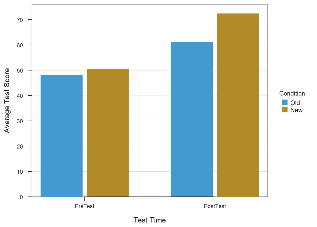
## Summary Table of Score
## ----------------------
##
##           Test
## Condition        PreTest      PostTest
##   Old             48.040        61.320
##   New             50.320        72.360
Alternatively, we can plot an interaction line plot using the interaction.plot function from base R.
interaction.plot(x.factor=df_long$Test,           # within-subjects variable
                 trace.factor=df_long$Condition,  # between-subjects variable
                 response=df_long$Score,          # outcome variable
                 fun=mean,                        # specify means be computed
                 type="b",                        # request lines and points
                 legend=TRUE,                     # request legend
                 pch=1,                           # request bubble points
                 ylab="Average Test Score",       # specify y-axis label
                 xlab="Test Time",                # specify x-axis label
                 trace.label="Condition")         # specify legend label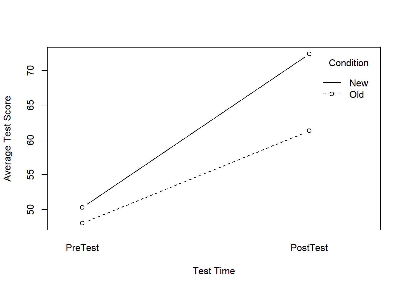
34.3.6 Estimating a Random-Coefficients Multilevel Model
Under these balanced-design conditions, a random-coefficients model (i.e., linear mixed-effects model, linear growth model, multilevel model) will also be statistically equivalent to a independent-samples t-test, simple linear regression model, biserial correlation with a difference score outcome variable, as well as a 2x2 mixed-factorial ANOVA model. We can also refer to this type of model as a linear growth model.
To estimate a random-coefficients model, we will use the lme function from the nlme package. If you haven’t already, please install and access the nlme package.
Using the <- assignment operator, we will assign our model to an object that we name lme_mod. To the right of the <- assignment operator, we will type the name of the lme model. As the first argument, we will type the name of the outcome variable (Score) followed by the ~ operator. As the second argument, we will type the name of the within-subjects/time-variant predictor variable (Test). As the third argument, we will type the name of the time-invariant/between-subjects variable (Condition). As the fourth argument, we will specify the interaction term between the time-variant and time-invariant variables using the * operator. As the fifth argument, we will insert random= followed by the ~ operator, the time-variant random-effects variable (Test), the | operator and the grouping variable (EmpID). As the sixth argument, we will specify data= followed by the name of the long-format data frame object (df_long). Finally, we will type the name of the summary function from base R with the sole parenthetical argument lme_mod to print a summary of the model results.
# Estimate random-coefficients multilevel model
lme_mod <- lme(Score ~                 # outcome variable (Score)
                 Test +                # time-variant variable (Test)
                 Condition +           # time-invariant variable (Condition)
                 Test * Condition,     # interaction term
               random= ~ Test |        # time-variant random-effects (Test)
                 EmpID,                # grouping variable (EmpID)
               data=df_long)           # data frame object name

# Print a summary of the model results
summary(lme_mod)
## Linear mixed-effects model fit by REML
## Data: df_long
## AIC BIC logLik
## 679.4852 700 -331.7426
##
## Random effects:
## Formula: ~Test | EmpID
## Structure: General positive-definite, Log-Cholesky parametrization
## StdDev Corr
## (Intercept) 5.776079 (Intr)
## TestPostTest 11.086832 -0.789
## Residual 3.313394
##
## Fixed effects: Score ~ Test + Condition + Test * Condition
## Value Std.Error DF t-value p-value
## (Intercept) 48.04 1.331791 48 36.07173 0.0000
## TestPostTest 13.28 2.407281 48 5.51660 0.0000
## ConditionNew 2.28 1.883437 48 1.21055 0.2320
## TestPostTest:ConditionNew 8.76 3.404409 48 2.57313 0.0132
## Correlation:
## (Intr) TstPsT CndtnN
## TestPostTest -0.767
## ConditionNew -0.707 0.543
## TestPostTest:ConditionNew 0.543 -0.707 -0.767
##
## Standardized Within-Group Residuals:
## Min Q1 Med Q3 Max
## -1.18371820 -0.30749376 -0.00838071 0.24550886 1.23636767
##
## Number of Observations: 100
## Number of Groups: 50When reviewing the estimated values associated with the fixed-effects interaction term between Test and Condition, we see the following: coefficient = 8.760, standard error = 3.404, t = 2.573, df = 48, and p = .0132. These values should look familiar. In fact, the coefficient value of 8.760 is the mean difference between the two “Old” and “New” conditions that we observed in the independent-samples t-test with a difference score outcome variable. The other estimate values should look familiar as well given that this random-coefficients multilevel model (i.e., growth model) is statistically equivalent to the other models we have estimated in this chapter.
To explore the model coefficient estimates further, let’s compute the cell means for our 2x2 pre-test/post-test with control group design by using the tapply function from base R.
- Type the name of the
tapplyfunction. - As the first argument in the
tapplyfunction, type the name of the data frame object (df_long) followed by the$operator and the name of the outcome variable containing the numeric data (Score):df_long$Score. - As the second argument in the
tapplyfunction, type the name of thelistfunction from base R.
- As the first argument, type the name of the data frame object (
df_long) followed by the$operator and the name of the first categorical variable (Test) from our model:df_long$Test. - As the first argument, type the name of the data frame object (
df_long) followed by the$operator and the name of the second categorical variable (Condition) from our model:df_long$Condition.
- As the third argument in the
tapplyfunction, type the name of themeanfunction from base R; doing so will compute the mean for each cell in the 2x2 cross-tabulation.
# Compute the cell means for the 2x2 cross-tabulation
tapply(df_long$Score,           # specify numeric outcome variable
       list(df_long$Test,       # specify first categorical variable
            df_long$Condition), # specify second categorical variable
       mean)                    # specify mean function
## Old New
## PreTest 48.04 50.32
## PostTest 61.32 72.36The 2x2 cross-tabulation produced in the output provides the mean score for each combination of crossed levels from the Test and Condition categorical variables. For example, the mean pre-test score for the “Old” condition is 48.04, and the mean post-test score for the “Old” condition is 61.32. With this table as an interpretation aid, let’s continue to unpack the results of the random-coefficients model we estimated above.
The intercept (
(Intercept)) estimate (i.e., value) of 48.04 represents the mean pre-test score for the “Old” training condition because, given the default reference groups (i.e., “PreTest” forTestvariable, “Old” forConditionvariable) the intercept represents mean test score when theTestPostTestdummy variable is equal to 0 (i.e., “PreTest”) and theConditionNewdummy variable is equal to 0 (i.e., “Old”).The
TestPostTestdummy variable estimate of 13.28 represents the difference between the mean post-test score and the mean pre-test score for the “Old” training condition (i.e., “PostTest” - “PreTest” for “Old” condition); given that the corresponding coefficient estimate is positive. Consequently, if we add 13.28 to 48.04, we arrive at 61.320, which represents the mean post-test score for those in the “Old” condition.The
ConditionNewdummy variable estimate of 2.28 represents the difference between the mean pre-test scores for the “New” and “Old” conditions (i.e., “New” - “Old” for “PreTest”). Given that the estimate is positive, it indicates that mean pre-test score for the “New” condition is slightly higher than that of the “Old” condition, but still more or less similar given the scaling of theTestvariable (i.e., can range from 0 to 100).Finally, as noted above, the estimate representing interaction between the
TestPostTestdummy variable andConditionNewdummy variable is equal to 8.76. This value represents the difference between the differences in mean post-test and pre-test scores between the “New” and “Old” conditions. In other words, the value of 8.76 represents the difference between mean post-test and pre-test scores for the “New” condition (72.36 - 50.32 = 22.04) minus the difference between mean post-test and pre-test scores for the “Old” condition (61.32 - 48.04 = 13.28), which equals 8.76 (22.04 - 13.28 = 8.76).
If we apply the anova function from base R to the fitted lme_mod object, we reproduce the results from our 2x2 mixed-factorial ANOVA model interaction term from the previous section. Specifically, please note the F-value and associated p-value for the Condition:Test line of the output.
##                numDF denDF  F-value p-value
## (Intercept)        1    48 8813.691  <.0001
## Test               1    48  107.636  <.0001
## Condition          1    48   24.688  <.0001
## Test:Condition     1    48    6.621  0.0132
Given the statistically significant interaction term between the between-subjects Condition variable and within-subjects Test variable, we will proceed forward with follow-up analyses of the between-subjects and within-subjects simple effects. Given our 2x2 design, our job examining the simple effects is made easier. Let’s begin with the between-subjects simple effects.
To compute the between-subjects simple effects, we will apply independent-samples t-tests to each level of the within-subjects factor. To do so, we will use the t.test function from base R.
- As the first argument, we’ll specify our model, which is our outcome variable (
Score) followed by the~operator and the predictor variable (Condition). - As the second argument, we’ll specify
data=followed by the name of our long-format data frame object (df_long). - As the third argument, we’ll specify
paired=FALSEto request an independent-samples t-test. - As the fourth argument, we’ll assume the variances are equal by applying
var.equal=TRUE. As the fifth argument, we’ll specifysubset=(Test=="PreTest")to filter the data down to just the “PreTest” scores. - We’ll then repeat the prior steps for the
PostTestscores in a separatet.testfunction.
# Between-subjects simple effects for the Condition variable
# by each level of the Test variable

# By PreTest level of Test variable
t.test(Score ~ Condition,
       data=df_long,
       paired=FALSE,
       var.equal=TRUE,
       subset=(Test=="PreTest"))
##
## Two Sample t-test
##
## data: Score by Condition
## t = -1.2106, df = 48, p-value = 0.232
## alternative hypothesis: true difference in means between group Old and group New is not equal to 0
## 95 percent confidence interval:
## -6.066903 1.506903
## sample estimates:
## mean in group Old mean in group New
## 48.04 50.32# By PostTest level of Test variable
t.test(Score ~ Condition,
data=df_long,
paired=FALSE,
var.equal=TRUE,
subset=(Test=="PostTest"))##
## Two Sample t-test
##
## data: Score by Condition
## t = -4.7976, df = 48, p-value = 0.000016
## alternative hypothesis: true difference in means between group Old and group New is not equal to 0
## 95 percent confidence interval:
## -15.666791 -6.413209
## sample estimates:
## mean in group Old mean in group New
## 61.32 72.36For the independent-samples t-test involving just the “PreTest” scores, we find that there is not a statistically significant difference for scores on the “PreTest” between the “New” and “Old” levels of the Condition variable (t = -1.2106, df = 48, p = .232). This tells us that those in the “New” and “Old” training conditions started at about the same place in terms of the scores prior to the training intervention.
For the independent-samples t-test involving just the “PostTest” scores, we find that there is a statistically significant difference for scores on the “PostTest” between the “New” and “Old” levels of the Condition variable (t = -4.7976, df = 48, p < .001). Examining the means informs us that those in the “New” training condition had statistically significantly higher scores on the “PostTest” than those in the “Old” training condition.
To compute the within-subjects simple effects, we will apply paired-samples t-tests to each level of the between-subjects fact. To do so, we will use the t.test function from base R once more.
- As the first argument, we’ll specify our model, which is our outcome variable (
Score) followed by the~operator and the predictor variable (Test). - As the second argument, we’ll specify
data=followed by the name of our long-format data frame object (df_long). - As the third argument, we’ll specify
paired=TRUEto request an paired-samples t-test. - As the fourth argument, we’ll specify
subset=(Condition=="Old")to filter the data down to just the “Old” condition scores. - We’ll then the previous steps for the “New” condition scores in a separate
t.testfunction.
# Within-subjects simple effects for the Test variable
# by each level of the Condition variable

# By Old level of Condition variable
t.test(Score ~ Test,
       data=df_long,
       paired=TRUE,
       subset=(Condition=="Old"))
##
## Paired t-test
##
## data: Score by Test
## t = -5.1935, df = 24, p-value = 0.00002548
## alternative hypothesis: true mean difference is not equal to 0
## 95 percent confidence interval:
## -18.55745 -8.00255
## sample estimates:
## mean difference
## -13.28# By Old level of Condition variable
t.test(Score ~ Test,
data=df_long,
paired=TRUE,
subset=(Condition=="New"))##
## Paired t-test
##
## data: Score by Test
## t = -9.8061, df = 24, p-value = 0.0000000007195
## alternative hypothesis: true mean difference is not equal to 0
## 95 percent confidence interval:
## -26.67877 -17.40123
## sample estimates:
## mean difference
## -22.04Both within-subjects simple effects show a statistically significant mean of the differences. If we combine this information with the table of means from our tapply function output (see above), we see that scores on both the “Old” condition and the “New” condition increased to a statistically significant extent from before to after training; however, the increase in scores for those in the “New” condition was notably larger.
When we find evidence of statistically significant interaction effects and simple effects, it often helps to visualize the results by creating a data visualization. Because we created a line chart in the previous section to display the same cell means from the 2x2 design, let’s mix things up by creating a bar chart. Specifically, let’s begin by using the BarChart function from the lessR package. If you haven’t already, be sure to install and access the lessR package using the install.packages and library functions, respectively.
# Create a bar chart
BarChart(x=Condition,                # between-subjects variable
         y=Score,                    # outcome variable
         by=Test,                    # within-subjects variable
         stat="mean",                # specify means be computed by category
         beside=TRUE,                # plot bars side-by-side
         values="input",             # add value labels representing cell means
         values_position="out",      # position value labels on top of bars
         fill=c("lightblue",         # specify dodgerblue for PreTest
                "darkblue"),         # specify lightgreen for PostTest
         data=df_long,               # name of data frame object
         xlab="Condition",           # specify x-axis title
         ylab="Average Test Score",  # specify y-axis title
legend_title="Test Time") # specify legend title 
## Summary Table of Score
## ----------------------
##
##     Condition
## Test              Old        New
##   PreTest      48.040     50.320
##   PostTest     61.320     72.360
Finally, to exert additional aesthetic and design control over our bar plot, we can use functions from the ggplot2 package. Before doing so, we need to aggregate our data using the summarize function from the dplyr package and the mean function from base R. If you haven’t already, be sure to install and access the dplyr and ggplot2 packages using the install.packages and library functions, respectively.
# Create a bar chart
df_long %>%                             # pipe in data frame object
  group_by(                             # group_by function
    Test,                               # 1st categorical predictor
    Condition                           # 2nd categorical predictor
    ) %>%                               # pipe to next function
  summarize(                            # summarize function
    Score=                              # new outcome var name
      mean(Score,                       # apply mean to outcome var
           na.rm=TRUE)                  # remove missing values
    ) %>%                               # pipe to next function
  ggplot(                               # ggplot function
    aes(                                # aes function
      x=Condition,                      # x-axis variable
      y=Score,                          # y-axis variable
      fill=Test)                        # legend/by variable
         ) +                            # add another element
  geom_bar(                             # geom_bar function
    stat="identity",                    # request original means
    position=position_dodge()           # side-by-side bars
    ) +                                 # add another element
  labs(                                 # labs function
    x="Condition",                      # x-axis title
    y="Average Test Score"              # y-axis title
    ) +                                 # add another element
  ylim(                                 # ylim function
    0,                                  # lower y-axis limit
    100                                 # lower y-axis limit
    ) +                                 # add another element
  geom_text(                            # geom_text function
    aes(                                # aes function
      label=Score),                     # value label variable
    position=position_dodge(width=0.9), # spacing of labels
    vjust=1.5,                          # labels just below bar tops
    color="white"                       # labels to white text
    ) +                                 # add another element
  theme_minimal(                        # theme_minimal function
  ) +                                   # add another element
  theme(                                # theme_minimal function
    panel.grid.major=element_blank(),   # remove major gridlines
    panel.grid.minor=element_blank()    # remove major gridlines
    ) +                                 # add another element
  scale_fill_brewer(                    # scale_fill_brewer function
    palette="Paired",                   # apply "Paired" palette
    name="Test Time")                   # legend title
## `summarise()` has grouped output by 'Test'. You can override using the `.groups` argument.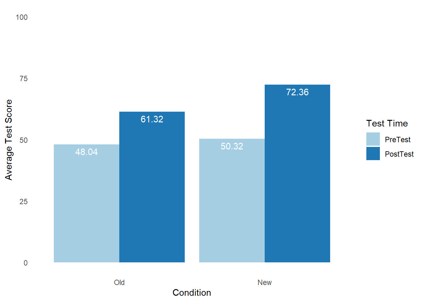
34.3.7 Estimating an Analysis of Covariance Model
When evaluating a randomized pre-test/post-test with control group design, there is another analysis that is not statistically equivalent to the other approaches but typically offers greater statistical power and estimation precision (Bodner and Bliese 2018). This approach involves the application of the analysis of covariance (ANCOVA) model, which does not allow us to directly infer whether change in scores from pre-test and post-test have occurred for either group; that is, the ANCOVA offers a less intuitive interpretation of the effects of a training program when compared to the approaches covered previous in the chapter.
Prior to estimating an ANCOVA, let’s re-order the default levels of the Condition variable from alphabetical (“New”, “Old”) to “Old” preceding “New”. This will ensure that the sign of the effect is comparable to what we found with the independent-samples t-test with a difference score outcome variable. To do so, we’ll convert the Condition variable to type factor using the factor function from base R. As the first argument, we’ll specify the name of the data frame object from the main portion of the chapter (df) followed by the $ operator and the name of the Condition variable. As the second argument, we’ll specify the levels= argument followed by the c function; as the two arguments within the c function, we’ll specify “Old” as the first argument and “New” as the second argument.
# Re-order Condition variable and convert to a factor
df$Condition <- factor(df$Condition,
                       levels=c("Old", "New"))
An ANCOVA model can be estimated using different functions and approaches. First, I’ll demonstrate how to estimate an ANCOVA using the aov and Anova functions from base R. This approach requires the car package, so be sure to install and access that package if you haven’t already.
To estimate an ANCOVA model, we’ll use the aov function from base R.
- Type the name of a new object that we can assign our model to using the
<-assignment operator. I’ve named the objectaov_modin this example. - Type the name of the
aovfunction.
- As the first argument, specify a model in which our post-test outcome variable (
PostTest) is regressed (~) onto our pre-test outcome variable (PreTest) and (+) our training group variable (Condition), which should look like this:PostTest ~ PreTest + Condition. - As the second argument, type the
data=argument followed by the name of the data frame object to which the variables in our model belong (`df).
- Type the name of the
Anovafunction from thecarpackage.
- As the first argument, type the name of the ANCOVA model we created based on the
aovfunction, which is (aov_mod). - As the second argument, type the
type=argument followed by “III” to request Type III sum of squares.
# Estimate an ANCOVA model
aov_mod <- aov(PostTest ~ PreTest + Condition,
               data=df)

# Request Type III sum of squares
Anova(aov_mod,
      type="III")
## Anova Table (Type III tests)
##
## Response: PostTest
## Sum Sq Df F value Pr(>F)
## (Intercept) 5681.4 1 93.4303 0.0000000000009477 ***
## PreTest 319.2 1 5.2486 0.02649 *
## Condition 1724.3 1 28.3559 0.0000027810204156 ***
## Residuals 2858.0 47
## ---
## Signif. codes: 0 '***' 0.001 '**' 0.01 '*' 0.05 '.' 0.1 ' ' 1The F-value associated with the Condition variable is 5.249, with a p-value of .026, which indicates that when controlling for the effects of the pre-test (PreTest), training group (Condition) is statistically significantly associated with the post-test (PostTest). What this finding does not tell us, however, is the direction of the association between Condition and PostTest when controlling for PreTest.
To figure out which training group performed better on the post-test when controlling for the pre-test, we will use the glht function from the multcomp package, so if you haven’t already installed and accessed the multcomp package, please do so first.
Type the name of the glht function and then do the following.
- Type the name of a new object that we can assign our model to using the
<-assignment operator. I’ve named the objectposthocin this example. - Type the name of the
glhtfunction.
- As the first argument, specify the name of the ANCOVA model object (
aov_mod). - As the second argument, type the
linfct=argument followed by themcpfunction. As the sole argument for themcpfunction, specify the name of the training group variable (Condition) followed by=and “Tukey”, where the latter requests Tukey’s pairwise comparisons that adjust for familywise error. Because we are only making a single comparison, the p-value will not be adjusted based on multiple comparisons. Still, it’s worthwhile getting used to this argument, especially if you plan to estimate an ANCOVA at some point in the future that involves three or more comparison groups.
# Estimate Tukey's post-hoc comparison test of mean difference
posthoc <- glht(aov_mod,
                linfct=mcp(Condition="Tukey"))

# Print summary of results
summary(posthoc)
##
## Simultaneous Tests for General Linear Hypotheses
##
## Multiple Comparisons of Means: Tukey Contrasts
##
##
## Fit: aov(formula = PostTest ~ PreTest + Condition, data = df)
##
## Linear Hypotheses:
## Estimate Std. Error t value Pr(>|t|)
## New - Old == 0 11.923 2.239 5.325 0.00000278 ***
## ---
## Signif. codes: 0 '***' 0.001 '**' 0.01 '*' 0.05 '.' 0.1 ' ' 1
## (Adjusted p values reported -- single-step method)In the output, we see that the null hypothesis being tested is New - Old == 0, which means that the default null hypothesis is that the means for the “New” and “Old” training programs are equal. This is typically what we want to test in this context. The estimated mean difference adjusted for pre-test (PreTest) scores is 11.923, and the associated p-value is less than .05. Another name for this adjusted mean is a conditional mean. The corresponding p-value should look familiar, as it is the same p-value we observed for the Condition variable in the ANCOVA model output. With the adjusted estimate of 11.923, we now know the direction of the effect. Specifically, because the value represents the mean for “New” minus the mean for “Old”, the positive 11.923 estimate indicates that post-test (PostTest) scores were, on average, higher for those in the “New” training group.
A statistically equivalent approach to estimating an ANCOVA model is to estimate a multiple linear regression model. To do so, we will use the lm function from base R.
- Type the name of a new object that we can assign our model to using the
<-assignment operator. I’ve named the objectlm_modin this example. - Type the
lmfunction.
- As the first argument, we’ll specify our model, which is the same model specification as our ANCOVA model above:
PostTest ~ PreTest + Condition - As the second argument, we’ll specify
data=followed by the name of the data frame object to which the variables in the model belong (df).
- Print a summary of the results using the
summaryfunction from base R with the name of our model object as the sole parenthetical argument (lm_mod).
# Estimate simple linear regression model
lm_mod <- lm(PostTest ~ PreTest + Condition,
             data=df)

# Print a summary of the model results
summary(lm_mod)
##
## Call:
## lm(formula = PostTest ~ PreTest + Condition, data = df)
##
## Residuals:
## Min 1Q Median 3Q Max
## -21.2717 -3.2743 0.6816 3.3986 18.8262
##
## Coefficients:
## Estimate Std. Error t value Pr(>|t|)
## (Intercept) 79.9230 8.2685 9.666 0.000000000000948 ***
## PreTest -0.3872 0.1690 -2.291 0.0265 *
## ConditionNew 11.9229 2.2390 5.325 0.000002781020416 ***
## ---
## Signif. codes: 0 '***' 0.001 '**' 0.01 '*' 0.05 '.' 0.1 ' ' 1
##
## Residual standard error: 7.798 on 47 degrees of freedom
## Multiple R-squared: 0.392, Adjusted R-squared: 0.3661
## F-statistic: 15.15 on 2 and 47 DF, p-value: 0.000008351In the output, the unstandardized regression coefficient associated with the ConditionNew variable is 11.923, and the p-value is less than .05, both of which are equal to the corresponding statistics found using the ANCOVA model and Tukey’s follow-up comparison. Because we set the reference group to “Old” for the Condition variable, the estimate of 11.923 represents the conditional mean difference between the “New” mean minus the “Old” mean, which is adjusted for pre-test (PreTest) scores. Thus, we can conclude that, when controlling for pre-test scores, those who participated in the “New” training group outperformed those who participated in the “Old” training group, on average. Finally, please note that unadjusted R-squared (R2) for the model is .392, which indicates that PreTest and Condition collectively explain 39.2% of the variance in PostTest.
To illustrate that conditional mean difference is in fact the difference between the conditional means, we can use the the emmeans function from the emmeans package. Please install and access the emmeans package, if you haven’t already.
To use the emmeans function, please do the following.
- Type the name of a new object that we can assign our conditional means to using the
<-assignment operator. I’ve named the objectcond_meansin this example. - Type the name of the
emmeansfunction.
- As the first argument, type the name of the linear regression model object (
lm_mod). - As the second argument, type the
specs=argument followed by the name of the training group variable (Condition). - As the third argument, type the
by=argument followed by the name of the pre-test variable (PreTest), which is the variable by which we are conditioning the means.
- Type the name of the
printfunction from base R with the conditional means object (cond_means) as the sole parenthetical argument.
# Estimate conditional means for PostTest
cond_means <- emmeans(lm_mod,
                      specs="Condition",
                      by="PreTest")

# Print the conditional means
print(cond_means)
## PreTest = 49.2:
## Condition emmean SE df lower.CL upper.CL
## Old 60.9 1.57 47 57.7 64
## New 72.8 1.57 47 69.6 76
##
## Confidence level used: 0.95In the output, the conditional mean for the “Old” training group is rounded to 60.9, and the conditional mean for the “New” training group is rounded to 72.8. To compute the difference between these two conditional means, we can extract the conditional mean for the focal group (“New”) and subtract from it the conditional mean for the reference group (“Old”). To do so, we will do the following.
- Create name for a new object (
df_cond_means) that will contain a data frame of conditional means using the<-assignment operator. - Type the name of the
summaryfunction from base R. As the sole parenthetical argument, type the name of the conditional means object created above (cond_means). - After the last parenthesis of the
summaryfunction, insert square brackets ([ ]).
- Within the square brackets (
[ ]), type a common (,). - To reference the column names from the
cond_meansobject, to the right of the comma (,) insert a vector of character column names using thecfunction. As the first argument, type the name of the training program variable (Condition) within quotation marks (" "). As the second argument, type the name of theemmeanobject containing from thecond_meansobject.
- On a new line, type the name of the
difffunction from base R. Within the function parenthesis, type the name of the newly createddf_cond_meansobject, followed by the$operator and theemmeanobject from thedf_cond_meansobject. This will extract the conditional means and the compute the difference.
# Create a table of just the conditional means and their Condition labels
df_cond_means <- summary(cond_means)[,c("Condition", "emmean")]

# Compute the difference between the conditional means
diff(df_cond_means$emmean)
## [1] 11.92291The resulting difference between the conditional means is 11.923 (after rounding), which should look very familiar, as it is the regression coefficient that we observed earlier associated with the Condition variable.
When we find statistically significant differences between conditional means, as we have in this instance, we often wish to create a data visualization to display the results. We can create a simple bar chart using the BarChart function from the lessR package. If you haven’t already, install and access the lessR package.
# Create a bar chart
BarChart(x=Condition,                         # training group variable
         y=emmean,                            # conditional means variable
         data=df_cond_means,                  # data frame object
         xlab="Training Condition",           # x-axis title
         ylab="Post-Test Conditional Means")  # y-axis title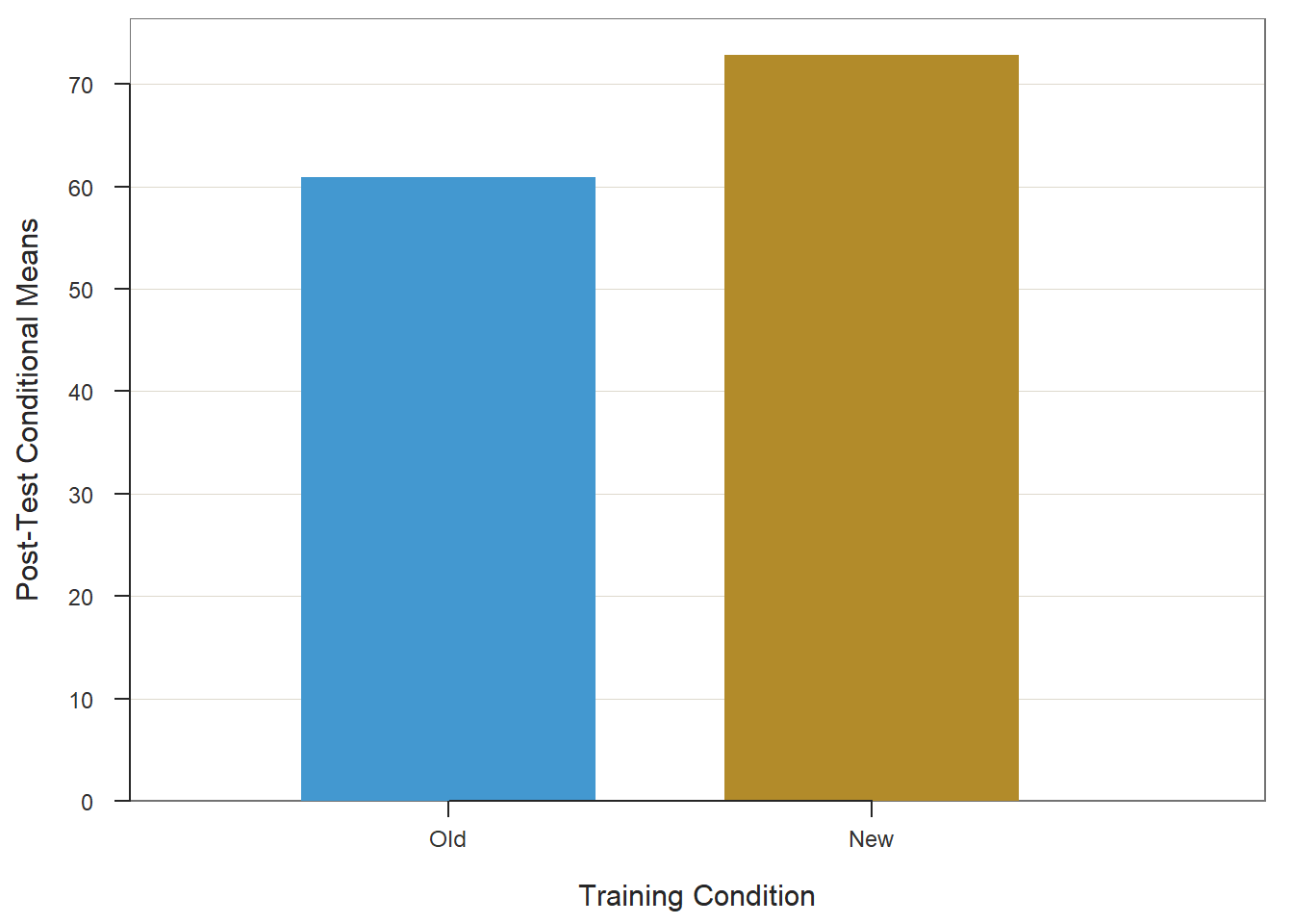
## >>> Suggestions
## Plot(emmean, Condition) # lollipop plot
##
##  Plotted Values
##  --------------
##      Old     New
##   60.879  72.801
If we wish to exert more aesthetic and stylistic control over our bar chart, we can use functions from the ggplot2 package as follows.
# Create a bar chart
ggplot(                                 # ggplot function
  df_cond_means,                        # data frame
  aes(                                  # aes function
    x=Condition,                        # x-axis variable
    y=emmean,                           # y-axis variable
    fill=Condition)                     # bar color variable
  ) +                                   # add another element
  geom_bar(                             # geom_bar function
    stat="identity",                    # request original means
    position=position_dodge()           # side-by-side bars
    ) +                                 # add another element
  labs(                                 # labs function
    x="Training Condition",             # x-axis title
    y="Post-Test Conditional Means"     # y-axis title
    ) +                                 # add another element
    ylim(                               # ylim function
    0,                                  # lower y-axis limit
    100                                 # lower y-axis limit
    ) +                                 # add another element
  geom_text(                            # geom_text function
    aes(                                # aes function
      label=round(emmean, 1)),          # rounded value label variable
    position=position_dodge(width=0.9), # spacing of labels
    vjust=1.5,                          # labels just below bar tops
    color="white"                       # labels to white text
    ) +                                 # add another element
  theme_minimal(                        # theme_minimal function
  ) +                                   # add another element
  theme(                                # theme_minimal function
    panel.grid.major=element_blank(),   # remove major gridlines
    panel.grid.minor=element_blank(),   # remove major gridlines
    legend.position="none")             # remove legend