Chapter 48 Identifying Predictors of Turnover Using Logistic Regression
In this chapter, we will learn how to estimate a (binary) logistic regression model in order to identify potential predictors of employee voluntary turnover, when voluntary turnover is operationalized as a dichotomous (i.e., binary) variable (e.g., stay vs. quit).
48.1 Conceptual Overview
Logistic regression (logit model) is part of the family of generalized linear models (GLMs). Assuming statistical assumptions have been satisfied, a binary logistic regression model is appropriate when the outcome variable of interest is dichotomous (i.e., binary) and when the predictor variable(s) of interest is/are continuous (interval, ratio) or categorical (nominal, ordinal). Unlike ordinary least squares (OLS) estimation, which was covered previously in the context of simple linear regression and multiple linear regression, logistic regression coefficients are typically estimated using maximum likelihood (ML). There are also extensions of the logistic regression like multinomial and ordinal logistic regression, where these extensions are appropriate when the categorical outcome variable is nominal or ordinal with three or more levels/categories.
Logistic regression can be used to determine the odds that a dichotomous event occurs (e.g., stay vs. quit) given higher or lower values/levels on one or more predictor variables, where odds refers to the probability of an event occurring (p) relative to the probability of the event not occurring (1 - p). As such, an odds value of 1 can be interpreted as 1 to 1 odds; or in other words, the probability of the event occurring is equal to the probability of the event not occurring, which would be akin to flipping a fair coin. For example, if we find that the probability of quitting is .75 (p = .75; i.e., event occurring), then by extension, the probability of not quitting is .25 (1 - p = .25; i.e., event not occurring). Given these probabilities, the odds of quitting are 3 (.75 / .25 = 3), and the odds of not quitting are 1/3 or .33, which is calculated as: .25 / (1 - .25). A logit transformation of the odds of quitting and of the odds of not quitting will be symmetrical, where a logit transformation refers to taking the natural log (\(\ln\)) of both values (i.e., logarithmic transformation). For example, a logit transformation of 3 and 1/3 yields 1.10 and -1.10, which are symmetrical: \(\ln(3) = 1.10\) and \(\ln(1/3) = -1.10\).
48.1.1 Review of Logistic Regression
Just as there is a distinction between simple and multiple linear regression models, we can also draw a distinction between simple and multiple logistic regression models. When there is a single predictor variable and a dichotomous outcome variable, we can apply what is referred to as a simple logistic regression model. More specifically, a simple logistic regression refers to the bivariate linear association between a predictor variable and a dichotomous outcome variable that has undergone a logit transformation, as shown in the equation below.
\(logit(p) = \log(odds) = \ln(\frac{p}{1-p}) = b_0 + b_1(X_1)\)
where \(logit(p)\) represents the logit transformation of the outcome, \(\log(odds)\) represents the log(arithmic) odds, \(\ln\) represents the natural log, \(p\) represents the probability of an event occurring, \(b_0\) represents the intercept value, and \(b_1\) represents the regression coefficient (i.e., slope, weight) of the association between the predictor variable \(X_1\) and the logit transformation of the outcome variable.
And when we have two or more predictor variables and a single dichotomous outcome variable, we estimate what is called a multiple logistic regression model, where an example of a multiple logistic regression model follows.
\(logit(p) = \log(odds) = \ln(\frac{p}{1-p}) = b_0 + b_1(X_1) + b_2(X_2)\)
where \(b_2\) represents the regression coefficient (i.e., slope, weight) of the association between the second predictor variable \(X_2\) and the logit transformation of the outcome variable.
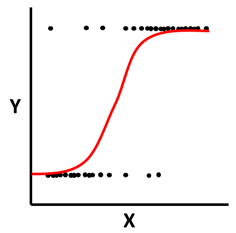
Logistic Function: Logistic regression is predicated on the logistic function. The scatter plot figure shown below illustrates the logistic function when there is a continuous (interval, ratio) predictor variable called \(X\) and a dichotomous outcome variable called \(Y\). Because a linear function would not not closely approximate the association between these two variables, we instead use a logistic function, which is a sigmoidal (or sigmoid) function and takes the visual form of an S-curve.
Just like simple and multiple linear regression models, regression coefficients are estimated in simple logistic regression models, but these coefficients are not perhaps as easily interpretable in their original form because the outcome variable undergoes a logarithmic transformation, as noted above. The regression coefficients in a logistic regression model represent the change in log odds (i.e., logit transformation) for every one unit change in the predictor variable.
Odds Ratio: To make a statistically significant regression coefficient (\(b_i\)) easier to interpret, we often convert the coefficient to an odds ratio. To do so, we exponentiate the coefficient using Euler’s number (\(e\)). Euler’s number (\(e\)) is an irrational number and mathematical constant that is approximately equal to 2.71828.
\(e^{b_i}\)
An odds ratio that is less than 1.00 indicates a negative association between the predictor variable and outcome variable, and an odds ratio that is greater than 1.00 indicates a positive association. An odds ratio equal to 1.00 indicates that there is no association between the variables.
Note: In the case of a multiple logistic regression model where we have two or more predictor variables, we would describe an odds ratios more accurately as an adjusted odds ratio because we are statistically controlling for the other predictor variable(s) in the model.
Example of Interpreting a Negative Association: As an example, let’s imagine in a simple logistic regression model we find that the coefficient for the association between job satisfaction (continuous predictor variable) and voluntary turnover (dichotomous outcome variable; i.e., stay = 0 vs. quit = 1) is -.42 – that is, we find a negative association. If we interpret the coefficient in its original form, we might say something like: “For every one unit increase in job satisfaction, there is as .42 unit reduction in log odds of quitting.” Such language will not typically be well-received by organizational stakeholders; however, if we convert the coefficient to an odds ratio by exponentiating it, we might find it easier to explain the finding to ourselves and others.
\(e^{-.42} = .66\)
In this example, the odds ratio of .66 is less than 1.00, which reflects back to us that the association is indeed negative, which we already knew from the original log odds coefficient value of -.42. We can interpret this odds ratio as follows: “For every unit increase in job satisfaction, the odds of quitting is reduced by 34% (1 - .66 = .34).” Alternatively, we can interpret the odds ratio from a different vantage point if we compute its reciprocal, which is 1.52 (1 / .66 = 1.52); in doing so, we can interpret the finding as: “For every unit increase in job satisfaction, the odds of quitting is reduced by 1 in 1.52.” Or, we could frame the finding in terms of not quitting: “For every unit increase in job satisfaction, the odds of not quitting is 1.52 times greater – or has a 1.52 times higher likelihood.”
Example of Interpreting a Positive Association: Now that we’ve worked through an example of a negative association, let’s practice interpreting a positive association. Let’s imagine a different simple logistic regression model in which we find that the coefficient for the association between turnover intentions (continuous predictor variable) and voluntary turnover (dichotomous outcome variable; i.e., stay = 0 vs. quit = 1) is .89. When interpreting the coefficient in its original form, we might say: “For every one unit increase in turnover intentions, there is as .89 unit increase in log odds of quitting.” Just as we did before, we can exponentiate the coefficient to find the odds ratio.
\(e^{.99} = 2.44\)
Because the odds ratio of 2.44 is greater than 1.00, it confirms to us that the association between turnover intentions and voluntary turnover is positive. We can interpret this finding as: “For every unit increase in turnover intentions, the odds of quitting is 2.44 times greater – or has a 2.44 times higher likelihood.”
As another example, let’s imagine that we observe an odds ratio of 1.29 with respect to negative affectivity in relation to voluntary turnover. We could interpret this finding as: “For every unit increase in negative affectivity, the odds of quitting is 1.29 times greater.” Or, because 1.29 times greater is equivalent to saying that there was a 29% increase, we could say: “For every unit increase in negative affectivity, the odds of quitting increases by 29%.”
Predicted Probabilities: Our logistic regression coefficients can also be used to predict the probability of the event occurring for different value(s) of the predictor variable(s). The equations that follow can help us to understand algebraically how we can determine the probability (\(p\)) of an event occurring based on the coefficients we might estimate for simple logistic regression model.
\(\ln(\frac{p}{1-p}) = b_0 + b_1(X_1)\)
\(\frac{p}{1-p} = e^{b_0 + b_1(X_1)}\)
\(p = \frac{e^{b_0 + b_1(X_1)}}{1+e^{b_0 + b_1(X_1)}}\)
where \(e\) represents Euler’s number.
As an example, let’s first imagine that our estimated intercept (\(b_0\)) is .32 and our estimated regression coefficient associated with the predictor variable (\(b_1\)) is -.09. Next, let’s imagine that someone has a score of 3 on the predictor variable (\(X_1\)). If we plug those values into the equation, we will find that the probability of a person with a score of 3 on the predictor variable is .51.
\(p = \frac{e^{b_0 + b_1(X_1)}}{1+e^{b_0 + b_1(X_1)}} = \frac{e^{.32 + (-.09 \times 3)}}{1+e^{.32 + (-.09 \times 3)}} = .51\)
If we set a probability threshold of .50 for experiencing the event, then we would classify anyone who scores a 3 on the predictor variable as having been predicted to experience the event in question. If however, the computed probability had been less than the probability threshold of .50, then we would have classified any associated with cases as having been predicted to not experience the event in question.
48.1.1.1 Statistical Assumptions
The statistical assumptions that should be met prior to running and/or interpreting estimates from a simple or multiple logistic regression model include:
- Cases are randomly sampled from the population, such that the variable scores for one individual are independent of the variable scores of another individual;
- Data are free of bivariate/multivariate outliers;
- The association between any continuous predictor variable(s) and the logit transformation of the outcome variable is linear;
- The outcome variable is dichotomous;
- For a multiple logistic regression model, there is no (multi)collinearity between predictor variables.
The fifth statistical assumption refers to the concept of collinearity (multicollinearity). This can be a tricky concept to understand, so let’s take a moment to unpack it. When two or more predictor variables are specified in a regression model, as is the case with multiple logistic regression, we need to be wary of collinearity. Collinearity refers to the extent to which predictor variables correlate with each other. Some level of intercorrelation between predictor variables is to be expected and is acceptable; however, if collinearity becomes substantial, it can affect the weights – and even the signs – of the regression coefficients in our model, which can be problematic from an interpretation standpoint. As such, we should avoid including predictors in a multiple linear regression model that correlate highly with one another. The tolerance statistic is commonly computed and serves as an indicator of collinearity. The tolerance statistic is computed by computing the shared variance (R2) of just the predictor variables in a single model (excluding the outcome variable), and subtracting that R2 value from 1 (i.e., 1 - R2). We typically grow concerned when the tolerance statistic falls below .20 and closer to .00. Ideally, we want the tolerance statistic to approach 1.00, as this indicates that there are lower levels of collinearity. From time to time, you might also see the variance inflation factor (VIF) reported as an indicator of collinearity; the VIF is just the reciprocal of the tolerance (i.e., 1/tolerance), and in my opinion, it is redundant to report and interpret both the tolerance and VIF. My recommendation is to focus just on the tolerance statistic when inferring whether the statistical assumption of no collinearity might have been violated.
Finally, with respect to the assumption that cases are randomly sampled from population, we will assume in this chapter’s data that this is not an issue. If we were to suspect, however, that there were some clustering or nesting of cases in units/groups (e.g., by supervisors, units, or facilities) with respect to our outcome variable, then we would need to run some type of multilevel model (e.g., multilevel logit model), which is beyond the scope of this tutorial. An intraclass correlation (ICC) can be used to diagnose such nesting or cluster. Failing to account for clustering or nesting in the data can bias estimates of standard errors, which ultimately influences the p-values and inferences of statistical significance.
48.1.1.2 Statistical Signficance
Using null hypothesis significance testing (NHST), we interpret a p-value that is less than .05 (or whatever two- or one-tailed alpha level we set) to meet the standard for statistical significance, meaning that we reject the null hypothesis that the regression coefficient is equal to zero. In other words, if a regression coefficient’s p-value is less than .05, we conclude that the regression coefficient differs from zero to a statistically significant extent. In contrast, if the regression coefficient’s p-value is equal to or greater than .05, then we fail to reject the null hypothesis that the regression coefficient is equal to zero. Put differently, if a regression coefficient’s p-value is equal to or greater than .05, we conclude that the regression coefficient does not differ from zero to a statistically significant extent, leading us to conclude that there is no association between the predictor variable and the outcome variable in the population. Keep in mind that in the context of a multiple logistic regression model, the association between each predictor variable and the logit transformation of the outcome variable must be interpreted with statistical control in mind, as we are effectively testing whether each predictor variable shows evidence of incremental validity in the presence of any other predictor variables.
When setting an alpha threshold, such as the conventional two-tailed .05 level, sometimes the question comes up regarding whether borderline p-values signify significance or nonsignificance. For our purposes, let’s be very strict in our application of the chosen alpha level. For example, if we set our alpha level at .05, p = .049 would be considered statistically significant, and p = .050 would be considered statistically nonsignificant.
Because our regression model estimates are based on data from a sample that is drawn from an underlying population, sampling error will affect the extent to which our sample is representative of the population from which its drawn. That is, a regression coefficient estimate (b) is a point estimate of the population parameter that is subject to sampling error. Fortunately, confidence intervals can give us a better idea of what the true population parameter value might be. If we apply an alpha level of .05 (two-tailed), then the equivalent confidence interval (CI) is a 95% CI. In terms of whether a regression coefficient is statistically significant, if the lower and upper limits of 95% CI do not include zero, then this tells us the same thing as a p-value that is less than .05. Strictly speaking, a 95% CI indicates that if we were to hypothetically draw many more samples from the underlying population and construct CIs for each of those samples, then the true parameter (i.e., true value of the regression coefficient in the population) would likely fall within the lower and upper bounds of 95% of the estimated CIs. In other words, the 95% CI gives us an indication of plausible values for the population parameter while taking into consideration sampling error. A wide CI (i.e., large difference between the lower and upper limits) signifies more sampling error, and a narrow CI signifies less sampling error.
Note: In a logistic regression model, we may also construct confidence intervals around the odds ratios.
48.1.1.3 Practical Significance
In its original form, a logistic regression coefficient is not an effect size; that is, it doesn’t provide an indication of practical significance. The odds ratio, however, can be conceptualized as an effect size. With that being said, there are some caveats. First, an odds ratio that is computed directly from an unstandardized logistic regression coefficient needs to be interpreted based on the raw scaling of the predictor variable, as the interpretation of the odds ratio has to do with the change in odds for unit change in the predictor variable. If we wish to compare odds ratios within or between models, we need to take this scaling issue into account. Second, in the case of a multiple logistic regression model, statistical control is at play, which means that the odds ratios are more accurately described as adjusted odds ratios.
There are different thresholds we can apply when interpreting the magnitude of an odds ratio, and below I provide some thresholds that we will use in this tutorial. With that being said, thresholds for qualitatively interpreting effect sizes should be context dependent, and there are other thresholds we might apply.
| Odds Ratio > 1 | Odds Ratio < 1 | Description |
|---|---|---|
| 1.2 | .8 | Small |
| 2.5 | .4 | Medium |
| 4.3 | .2 | Large |
At the model level, we can’t compute a true R2 when estimating a logistic regression model. We can, however, compute a pseudo-R2, There are different formulas available for computing pseudo-R2 (e.g., Cox & Snell, McFadden), and in this chapter we’ll focus on the following Nagelkerke (1991) formula:
\(pseudo-R^2 = \frac{1 - (\frac{L(M_{null})}{L(M_{full})})^{2/N}}{1-L(M_{null})^{2/N}}\)
where \(L(M_{null})\) is the likelihood of the outcome variable given a null, intercept-only model, \(L(M_{full})\) is the likelihood of the outcome variable given the predictor variable(s) in the model, and \(N\) is the sample size.
It’s important to note, though, that as the name implies, a pseudo-R2 is not the same thing as a true R2. Thus, while we need to be cautious in our interpretations.
In addition to pseudo-R2, we can also describe the classification accuracy of the model by using a confusion matrix (or classification table). A confusion matrix presents the percentage of correctly predicted values on the outcome variable; if a probability for a case based on the model is equal to or greater than .50, then it would be classified as a probability of 1, and all else would be classified as 0. For example, using a confusion matrix, we can make statements like: “The model correctly classified 55.9% of the employees as either stay or quit.”
To indicate how well your model fit the data and performed, I recommend reporting either pseudo-R2, model classification accuracy, or both.
Note: Typically, we only interpret the practical significance of an effect if the effect was found to be statistically significant. The logic is that if an effect (e.g., association, difference) is not statistically significant, then we should treat it as no different than zero, and thus it wouldn’t make sense to the interpret the size of something that statistically has no effect.
48.1.1.4 Sample Write-Up
A voluntary turnover study was conducted based on a sample 99 employees from the past year, some of whom quit the company and some of whom stayed. The focal outcome variable is turnover behavior (quit vs. stay), and because it is dichotomous, we used logistic regression. We were, specifically, interested in the extent to which employees’ self-reported job satisfaction, negative affectivity, and turnover intentions were associated with their decisions to quit or stay, and thus all three were was used as continuous predictor variables in our multiple logistic regression model. In total, due to missing data, 95 employees were included in our analysis. Results indicated that job satisfaction was not associated with turnover behavior to a statistically significant extent (b = -.233, p = .293, 95% CI[-.667, .201]). Negative affectivity, however, was positively and significantly associated with turnover behavior (b = 1.195, p = .017, 95% CI[.216, 2.174]). For every one unit increase in negative affectivity, the odds of quitting were 3.304 times greater, when controlling for the other predictor variables in the model. Similarly, turnover intentions were also positively and significantly associated with turnover behavior (b = .897, p = .005, 95% CI[.276, 1.517]). For every one unit increase in turnover intentions, the odds of quitting were 2.451 times greater, when controlling for other predictor variables in the model. Both of these significant associations can be described as medium in magnitude. Overall, based on our estimated multiple logistic regression model, we were able to correct classify 78.9% of employees from our sample using the estimated multiple logistic regression model. Finally, the estimated Nagelkerke pseudo-R2 was .073. We can cautiously conclude that job satisfaction explains 7.3% of the variance in voluntary turnover.
48.2 Tutorial
This chapter’s tutorial demonstrates how to estimate simple and multiple logistic regression models using R.
48.2.1 Video Tutorials
As usual, you have the choice to follow along with the written tutorial in this chapter or to watch the video tutorial below.
Link to video tutorial: https://youtu.be/O7gRceyeyT8
48.2.2 Functions & Packages Introduced
| Function | Package |
|---|---|
Logit |
lessR |
log |
base R |
PseudoR2 |
DescTools |
exp |
base R |
glm |
base R |
merge |
base R |
data.frame |
base R |
mutate |
dplyr |
ifelse |
base R |
c |
base R |
predict |
base R |
detach |
base R |
48.2.3 Initial Steps
If you haven’t already, save the file called “Turnover.csv” into a folder that you will subsequently set as your working directory. Your working directory will likely be different than the one shown below (i.e., "H:/RWorkshop"). As a reminder, you can access all of the data files referenced in this book by downloading them as a compressed (zipped) folder from the my GitHub site: https://github.com/davidcaughlin/R-Tutorial-Data-Files; once you’ve followed the link to GitHub, just click “Code” (or “Download”) followed by “Download ZIP”, which will download all of the data files referenced in this book. For the sake of parsimony, I recommend downloading all of the data files into the same folder on your computer, which will allow you to set that same folder as your working directory for each of the chapters in this book.
Next, using the setwd function, set your working directory to the folder in which you saved the data file for this chapter. Alternatively, you can manually set your working directory folder in your drop-down menus by going to Session > Set Working Directory > Choose Directory…. Be sure to create a new R script file (.R) or update an existing R script file so that you can save your script and annotations. If you need refreshers on how to set your working directory and how to create and save an R script, please refer to Setting a Working Directory and Creating & Saving an R Script.
Next, read in the .csv data file called “Turnover.csv” using your choice of read function. In this example, I use the read_csv function from the readr package (Wickham, Hester, and Bryan 2024). If you choose to use the read_csv function, be sure that you have installed and accessed the readr package using the install.packages and library functions. Note: You don’t need to install a package every time you wish to access it; in general, I would recommend updating a package installation once ever 1-3 months. For refreshers on installing packages and reading data into R, please refer to Packages and Reading Data into R.
# Install readr package if you haven't already
# [Note: You don't need to install a package every
# time you wish to access it]
install.packages("readr")
# Access readr package
library(readr)
# Read data and name data frame (tibble) object
td <- read_csv("Turnover.csv")## Rows: 99 Columns: 6
## ── Column specification ────────────────────────────────────────────────────────────────────────────────────────────────────────────
## Delimiter: ","
## chr (1): ID
## dbl (5): Turnover, JS, OC, TI, NAff
##
## ℹ Use `spec()` to retrieve the full column specification for this data.
## ℹ Specify the column types or set `show_col_types = FALSE` to quiet this message.## [1] "ID" "Turnover" "JS" "OC" "TI" "NAff"## spc_tbl_ [99 × 6] (S3: spec_tbl_df/tbl_df/tbl/data.frame)
## $ ID : chr [1:99] "EMP559" "EMP561" "EMP571" "EMP589" ...
## $ Turnover: num [1:99] 1 1 1 1 1 1 0 1 1 1 ...
## $ JS : num [1:99] 4.96 1.72 1.64 3.01 3.04 3.81 1.38 3.92 2.35 1.69 ...
## $ OC : num [1:99] 5.32 1.47 0.87 2.15 1.94 3.81 0.83 3.88 3.03 2.82 ...
## $ TI : num [1:99] 0.51 4.08 2.65 4.17 3.27 3.01 3.18 1.7 2.44 2.58 ...
## $ NAff : num [1:99] 1.87 2.48 2.84 2.43 2.76 3.67 2.3 2.8 2.71 2.07 ...
## - attr(*, "spec")=
## .. cols(
## .. ID = col_character(),
## .. Turnover = col_double(),
## .. JS = col_double(),
## .. OC = col_double(),
## .. TI = col_double(),
## .. NAff = col_double()
## .. )
## - attr(*, "problems")=<externalptr>## # A tibble: 6 × 6
## ID Turnover JS OC TI NAff
## <chr> <dbl> <dbl> <dbl> <dbl> <dbl>
## 1 EMP559 1 4.96 5.32 0.51 1.87
## 2 EMP561 1 1.72 1.47 4.08 2.48
## 3 EMP571 1 1.64 0.87 2.65 2.84
## 4 EMP589 1 3.01 2.15 4.17 2.43
## 5 EMP592 1 3.04 1.94 3.27 2.76
## 6 EMP601 1 3.81 3.81 3.01 3.67There are 5 variables and 99 cases (i.e., employees) in the td data frame: ID, Turnover, JS, OC, TI, and NAff. Per the output of the str (structure) function above, all of the variables are of type numeric (continuous: interval/ratio), except for the ID variable, which is of type character. ID is the unique employee identifier variable. Imagine that these data were collected as part of a turnover study within an organization to determine the drivers/predictors of turnover based on a sample of employees who stayed and leaved during the past year. The variables JS, OC, TI, and NAff were collected as part of an annual survey and were later joined with the Turnover variable. Survey respondents rated each survey item using a 7-point response scale, ranging from strongly disagree (0) to strongly agree (6). JS contains the average of each employee’s responses to 10 job satisfaction items. OC contains the average of each employee’s responses to 7 organizational commitment items. TI contains the average of each employee’s responses to 3 turnover intentions items, where higher scores indicate higher levels of turnover intentions. NAff contains the average of each employee’s responses to 10 negative affectivity items. Turnover is a variable that indicates whether these individuals left the organization during the prior year, with 1 = quit and 0 = stayed. Note: If the Turnover variable were to include the character values of quit and stay instead of 1 and 0, the functions covered in this tutorial would automatically convert the character values to 0 and 1 (behind the scenes), where 0 would be assigned to the character value that comes first alphabetically.
48.2.4 Estimate Simple Logistic Regression Model
We’ll begin by specifying a simple logistic regression model, which means the model will include just one predictor variable. Let’s begin by regressing Turnover on JS using the Logit function from the lessR package (Gerbing, Business, and University 2021). If you haven’t already, install and access the lessR package.
As the first argument in the Logit function, specify the logistic regression model, wherein the dichotomous outcome variable is typed to the left of the ~ symbol, and the predictor variable is typed to the right of the ~ symbol. As the second argument, type data= followed by the name of the data frame to which both of the variables belong (td). Let’s begin by specifying JS as the predictor variable.
##
## Response Variable:   Turnover
## Predictor Variable 1:  JS
##
## Number of cases (rows) of data:  99
## Number of cases retained for analysis:  98
##
##
##    BASIC ANALYSIS
##
## -- Estimated Model of Turnover for the Logit of Reference Group Membership
##
##              Estimate    Std Err  z-value  p-value   Lower 95%   Upper 95%
## (Intercept)    1.8554     0.6883    2.695    0.007      0.5063      3.2044
##          JS   -0.4378     0.1958   -2.236    0.025     -0.8216     -0.0540
##
##
## -- Odds Ratios and Confidence Intervals
##
##              Odds Ratio   Lower 95%   Upper 95%
## (Intercept)      6.3939      1.6591     24.6415
##          JS      0.6455      0.4397      0.9475
##
##
## -- Model Fit
##
##     Null deviance: 131.746 on 97 degrees of freedom
## Residual deviance: 126.341 on 96 degrees of freedom
##
## AIC: 130.3413
##
## Number of iterations to convergence: 4
##
##
##    ANALYSIS OF RESIDUALS AND INFLUENCE
## Data, Fitted, Residual, Studentized Residual, Dffits, Cook's Distance
##    [sorted by Cook's Distance]
##    [res_rows = 20 out of 98 cases (rows) of data]
## --------------------------------------------------------------------
##      JS Turnover fitted residual rstudent  dffits   cooks
## 69 6.00        1 0.3162   0.6838   1.5688  0.3725 0.08496
## 7  1.38        0 0.7775  -0.7775  -1.7682 -0.2877 0.06241
## 73 5.48        1 0.3673   0.6327   1.4476  0.2949 0.04889
## 58 5.43        1 0.3724   0.6276   1.4363  0.2877 0.04618
## 12 1.72        0 0.7507  -0.7507  -1.6920 -0.2486 0.04353
## 31 1.77        0 0.7466  -0.7466  -1.6810 -0.2429 0.04117
## 13 1.96        0 0.7305  -0.7305  -1.6393 -0.2219 0.03314
## 1  4.96        1 0.4217   0.5783   1.3332  0.2239 0.02609
## 33 4.88        1 0.4302   0.5698   1.3162  0.2138 0.02353
## 84 4.66        1 0.4540   0.5460   1.2703  0.1875 0.01757
## 63 4.65        1 0.4551   0.5449   1.2682  0.1863 0.01733
## 61 2.52        0 0.6797  -0.6797  -1.5199 -0.1668 0.01693
## 97 5.59        0 0.3562  -0.3562  -0.9554 -0.2021 0.01693
## 70 5.48        0 0.3673  -0.3673  -0.9731 -0.1985 0.01648
## 74 2.56        0 0.6758  -0.6758  -1.5115 -0.1635 0.01615
## 75 2.57        0 0.6749  -0.6749  -1.5095 -0.1626 0.01596
## 67 2.65        0 0.6671  -0.6671  -1.4929 -0.1563 0.01454
## 80 5.04        0 0.4131  -0.4131  -1.0457 -0.1813 0.01431
## 77 4.46        1 0.4757   0.5243   1.2296  0.1656 0.01336
## 39 4.43        1 0.4790   0.5210   1.2235  0.1625 0.01282
##
##
##    PREDICTION
##
## Probability threshold for classification : 0.5
##
##
## Data, Fitted Values, Standard Errors
##    [sorted by fitted value]
##    [pred_all=TRUE to see all intervals displayed]
## --------------------------------------------------------------------
##      JS Turnover label fitted std.err
## 69 6.00        1     0 0.3162  0.1215
## 97 5.59        0     0 0.3562  0.1120
## 70 5.48        0     0 0.3673  0.1090
## 73 5.48        1     0 0.3673  0.1090
##
## ... for the rows of data where fitted is close to 0.5 ...
##
##      JS Turnover label fitted std.err
## 39 4.43        1     0 0.4790 0.07497
## 83 4.41        0     0 0.4812 0.07431
## 64 4.26        1     0 0.4976 0.06946
## 27 4.15        0     1 0.5097 0.06609
## 14 4.14        0     1 0.5107 0.06579
##
## ... for the last 4 rows of sorted data ...
##
##      JS Turnover label fitted std.err
## 66 1.19        1     1 0.7916 0.07790
## 48 1.05        1     1 0.8015 0.07904
## 88 0.67        1     1 0.8266 0.08096
## 24 0.23        1     1 0.8525 0.08116
## --------------------------------------------------------------------
##
##
## ----------------------------
## Specified confusion matrices
## ----------------------------
##
## Probability threshold for predicting : 0.5
## Corresponding cutoff threshold for JS: 4.238
##
##                  Baseline         Predicted
## ---------------------------------------------------
##                 Total  %Tot        0      1  %Correct
## ---------------------------------------------------
##            1       59  60.2       10     49     83.1
## Turnover   0       39  39.8        8     31     20.5
## ---------------------------------------------------
##          Total     98                           58.2
##
## Accuracy: 58.16
## Sensitivity: 83.05
## Precision: 61.25
Note: In some instances, you might receive an error message like the one shown below. You can ignore such a message, as it just indicates that you have a very poor-performing model that results in predicted outcome-variable classifications that are all the same (e.g., all of the predicted values are 0). If you receive such a message, you can proceed forward with your interpretation of the output.
\(\color{red}{\text{Error:}}\) \(\color{red}{\text{All predicted values are 0.}}\) \(\color{red}{\text{Something is wrong here.}}\)
The output generates the model coefficient estimates, the odds ratios and their confidence intervals, model fit information (i.e., AIC), outlier detection, forecasts, and a confusion matrix. At the top of the output, we get information about which variables were included in our model (which we probably already knew), the number of cases (e.g., employees) in the data, and the number of cases retained for the analysis after excluding cases with missing data (N = 98).
48.2.4.1 Test Statistical Assumptions
To determine whether it’s appropriate to interpret the results of a simple logistic regression model, we need to first test the following statistical assumptions.
Cases Are Randomly Sampled from the Population: As mentioned in the statistical assumptions section, we will assume that the cases (i.e., employees) were randomly sampled from the population, and thus conclude that this assumption has been satisfied.
Outcome Variable Is Dichotomous: We already know that the outcome variable called Turnover is dichotomous (1 = quit, 0 = stayed), which means we have satisfied this assumption.
Data Are Free of Bivariate Outliers: To determine whether the data are free of bivariate outliers, let’s take a look at the text output section called Analysis of Residuals and Influence. We should find a table with a unique identifiers column (that shows the row number in your data frame object), the observed (actual) predictor and outcome variable values, the fitted (predicted) outcome variable values, the residual (error) between the fitted values and the observed outcome variable values, and the following three outlier/influence statistics: Studentized residual (rstdnt), number of standard error units that a fitted value shifts when the flagged case is removed (dffits), and Cook’s distance (cooks). The case associated with row number 66 has the highest Cook’s distance value (.085), followed by the cases associated with row numbers 67 and 71, which have Cook’s distance values of .062 and .049. A liberal threshold Cook’s distance is 1, which means that we would grow concerned if any of these values exceeded 1, whereas a more conservative threshold is 4 divided by the sample size (4 / 98 = .041). As a sensitivity analysis, we may want to estimate our model once more after removing the cases associated with row numbers 66, 66, and 71 from our data frame; however, these Cook’s distance values don’t look too concerning or out of the ordinary, and thus I wouldn’t recommend removing the associated cases. In general, we should be wary of removing outliers or influential cases and should do so only when we have a very strong justification for doing so.
Association Between Any Continuous Predictor Variable and Logit Transformation of Outcome Variable Is Linear: To test the assumption of linearity between a continuous predictor variable and the logit transformation of the outcome variable, we can add the interaction between the predictor variable and its logarithmic (i.e., natural log) transformation. [Note: We do not perform the following test/approach for categorical predictor variables.] We will use an approach that is commonly referred to as the Box-Tidwell approach (Hosmer and Lemeshow 2000). To apply this approach, we need to add the interaction term between our predictor variable JS and its logarithmic transformation to our logistic regression model – but not the main effect for the logarithmic transformation of JS. In our regression model formula, specify the dichotomous outcome variable Turnover to the left of the ~ operator. To the right of the ~ operator, type the name of the predictor variable JS followed by the + operator. After the + operator, type the name of the predictor variable JS, followed by the : operator and the log function from base R with the predictor variable JS as its sole parenthetical argument.
# Box-Tidwell diagnostic test of linearity between continuous predictor variable and
# logit transformation of outcome variable
Logit(Turnover ~ JS + JS:log(JS), data=td)
##
## Response Variable: Turnover
## Predictor Variable 1: JS
##
## Number of cases (rows) of data: 99
## Number of cases retained for analysis: 98
##
##
## BASIC ANALYSIS
##
## -- Estimated Model of Turnover for the Logit of Reference Group Membership
##
## Estimate Std Err z-value p-value Lower 95% Upper 95%
## (Intercept) 5.4461 3.2062 1.699 0.089 -0.8379 11.7300
## JS -2.9840 2.1693 -1.376 0.169 -7.2357 1.2677
## JS:log(JS) 1.1696 0.9778 1.196 0.232 -0.7467 3.0860
##
##
## -- Odds Ratios and Confidence Intervals
##
## Odds Ratio Lower 95% Upper 95%
## (Intercept) 231.8457 0.4326 124248.7675
## JS 0.0506 0.0007 3.5527
## JS:log(JS) 3.2208 0.4739 21.8896
##
##
## -- Model Fit
##
## Null deviance: 131.746 on 97 degrees of freedom
## Residual deviance: 124.621 on 95 degrees of freedom
##
## AIC: 130.6211
##
## Number of iterations to convergence: 5
##
##
## ANALYSIS OF RESIDUALS AND INFLUENCE
## Data, Fitted, Residual, Studentized Residual, Dffits, Cook's Distance
## [sorted by Cook's Distance]
## [res_rows = 20 out of 98 cases (rows) of data]
## --------------------------------------------------------------------
## JS Turnover fitted residual rstudent dffits cooks
## 7 1.38 0 0.8639 -0.8639 -2.105 -0.4827 0.158262
## 69 6.00 1 0.5290 0.4710 1.221 0.5442 0.090322
## 12 1.72 0 0.8029 -0.8029 -1.852 -0.3440 0.063819
## 31 1.77 0 0.7936 -0.7936 -1.821 -0.3267 0.055946
## 97 5.59 0 0.5044 -0.5044 -1.239 -0.3947 0.049267
## 73 5.48 1 0.4993 0.5007 1.224 0.3561 0.039962
## 70 5.48 0 0.4993 -0.4993 -1.221 -0.3554 0.039735
## 58 5.43 1 0.4972 0.5028 1.224 0.3418 0.036908
## 13 1.96 0 0.7577 -0.7577 -1.713 -0.2696 0.034590
## 80 5.04 0 0.4853 -0.4853 -1.174 -0.2378 0.017543
## 1 4.96 1 0.4840 0.5160 1.225 0.2327 0.017368
## 33 4.88 1 0.4830 0.5170 1.225 0.2184 0.015319
## 61 2.52 0 0.6572 -0.6572 -1.476 -0.1788 0.012429
## 74 2.56 0 0.6506 -0.6506 -1.462 -0.1758 0.011886
## 75 2.57 0 0.6490 -0.6490 -1.459 -0.1751 0.011761
## 84 4.66 1 0.4823 0.5177 1.221 0.1854 0.011051
## 63 4.65 1 0.4823 0.5177 1.221 0.1842 0.010899
## 67 2.65 0 0.6363 -0.6363 -1.433 -0.1701 0.010877
## 96 2.82 0 0.6108 -0.6108 -1.384 -0.1623 0.009530
## 21 4.64 0 0.4824 -0.4824 -1.159 -0.1737 0.009334
##
##
## PREDICTION
##
## Probability threshold for classification : 0.5
##
##
## Data, Fitted Values, Standard Errors
## [sorted by fitted value]
## [pred_all=TRUE to see all intervals displayed]
## --------------------------------------------------------------------
## JS Turnover label fitted std.err
## 84 4.66 1 0 0.4823 0.08526
## 63 4.65 1 0 0.4823 0.08471
## 21 4.64 0 0 0.4824 0.08416
## 53 4.63 0 0 0.4824 0.08363
##
## ... for the rows of data where fitted is close to 0.5 ...
##
## JS Turnover label fitted std.err
## 70 5.48 0 0 0.4993 0.15604
## 73 5.48 1 0 0.4993 0.15604
## 55 3.97 1 1 0.5005 0.06559
## 16 3.95 0 1 0.5015 0.06547
## 8 3.92 1 1 0.5031 0.06531
##
## ... for the last 4 rows of sorted data ...
##
## JS Turnover label fitted std.err
## 66 1.19 1 1 0.8945 0.08584
## 48 1.05 1 1 0.9147 0.08191
## 88 0.67 1 1 0.9582 0.06150
## 24 0.23 1 1 0.9874 0.02972
## --------------------------------------------------------------------
##
##
## ----------------------------
## Specified confusion matrices
## ----------------------------
##
## Probability threshold for predicting : 0.5
## Corresponding cutoff threshold for JS: 1.825
##
## Baseline Predicted
## ---------------------------------------------------
## Total %Tot 0 1 %Correct
## ---------------------------------------------------
## 1 59 60.2 9 50 84.7
## Turnover 0 39 39.8 14 25 35.9
## ---------------------------------------------------
## Total 98 65.3
##
## Accuracy: 65.31
## Sensitivity: 84.75
## Precision: 66.67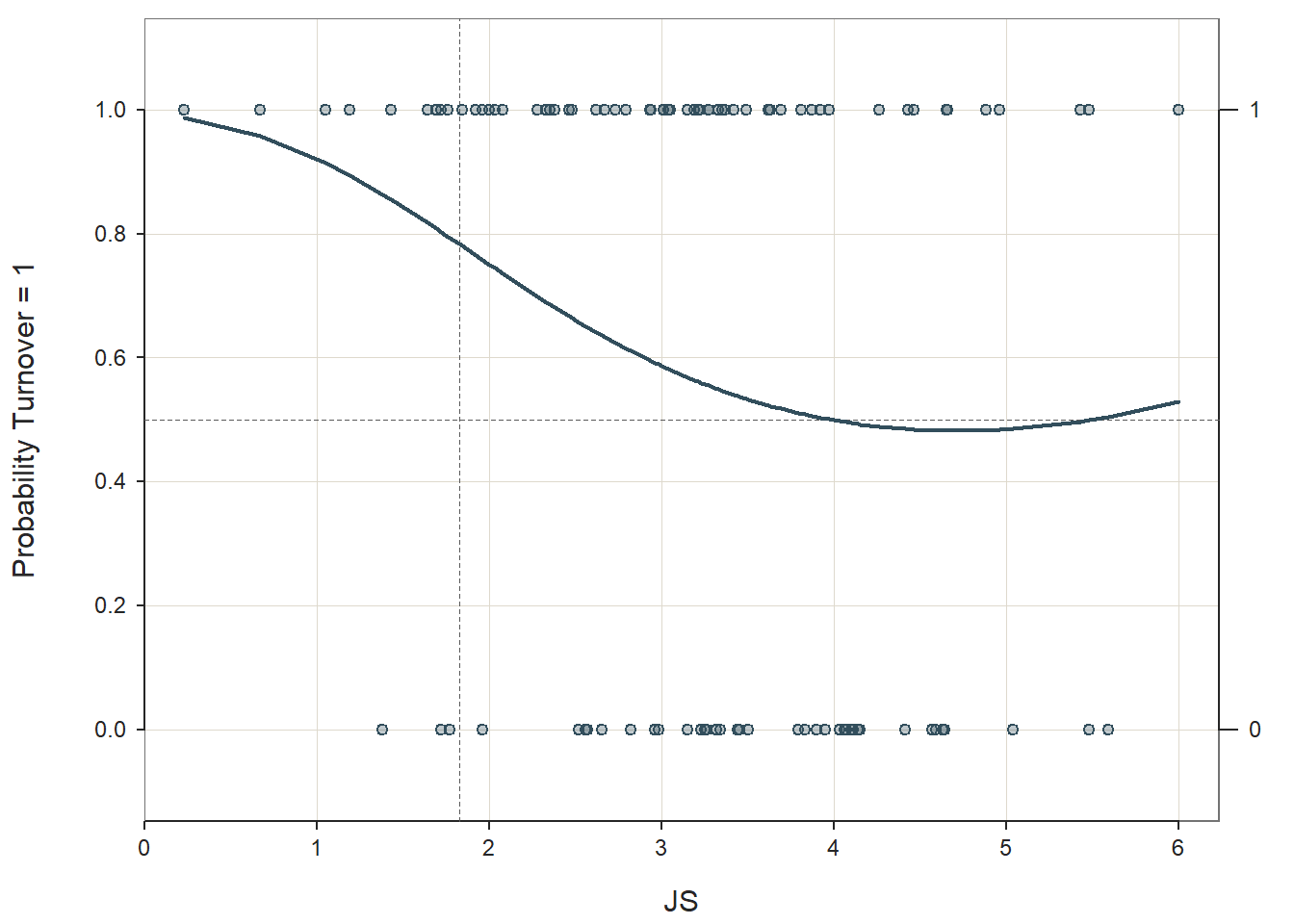
Because the interaction term (JS:log(JS)) regression coefficient of 1.1696 in the Model Coefficients table is nonsignificant (p = .232), we have no reason to believe that the association between the continuous predictor variable and the logit transformation of the outcome variable is nonlinear. If the interaction term had been statistically significant, then we might have evidence that the assumption was violated, and one potential solution would be to estimate a polynomial model of some kind to better fit the data; for more information on estimating nonlinear associations, check out Chapter 7 (“Curvilinear Effects in Logistic Regression”) from Osborne (2015). Finally, we only apply this test when the predictor variable in question is continuous (interval, ratio). In practice, however, note that for reasons of parsimony, we sometimes we might choose to estimate a linear model over a nonlinear/polynomial model when the former fits the data reasonably well.
Important Note: If the variable for which you are applying the Box-Tidwell approach described above has one or more cases with a score of zero, then you will receive an error message when you run the model with the log function. The reason for the error is that the log of zero or any negative value is (mathematically) undefined. There are many reasons why your variable might have cases with scores equal to zero, some of which include: (a) zero is a naturally occurring value for the scale on which the variable is based, or (b) the variable was grand-mean centered or standardized, such that the mean is now equal to zero. There are some approaches to dealing with this issue and neither approach I will show you is going to be perfect, but each approach will give you an approximate understanding of whether violation of the linearity assumption might be an issue. First, we can add a positive numeric constant to every score on the continuous predictor variable in question that will result in the new lowest score being 1. Why 1 you might ask? Well, the rationale is somewhat arbitrary; the log of 1 is zero, and there is something nice about grounding the lowest logarithmic value at 0. Due note, however, that the magnitude of the linear transformation will have some effect on the p-value associated with the Box-Tidwell interaction term. Second, if there are proportionally very few cases with scores of zero on the predictor variable in question, we can simply subset those cases out for the analysis.
Just for the sake of demonstration, let’s transform the JS variable so that its lowest score is equal to zero. This will give us an opportunity to test the two approaches I described above. Simply, create a new variable (JS_0) that is equal to JS minus the minimum value of JS.
# ONLY FOR DEMONSTRATION PURPOSES: Create new predictor variable where lowest score is zero
td$JS_0 <- td$JS - min(td$JS, na.rm=TRUE)
Now that we have a variable called JS_0 with at least one score equal to zero, let’s try the try the Box-Tidwell test. I’m going to add the argument brief=TRUE to reduce the amount of output generated by the function.
# Box-Tidwell diagnostic test of linearity between continuous predictor variable and
# logit transformation of outcome variable [with predictor containing zero value(s)]
Logit(Turnover ~ JS_0 + JS_0:log(JS_0), data=td, brief=TRUE)
If you ran the script above, you likely got an error message that looked like this:
\(\color{red}{\text{Error in glm.fit(x = c(1, 1, 1, 1, 1, 1, 1, 1, 1, 1, 1, 1, 1, 1, 1, 1, : NA/NaN/Inf in 'x'}}\)
The reason we got this error message is because the log of zero is undefined, and because we had at least one case with a value of zero on JS_0, it broke down the operations. If you see a message like that, then proceed with one or both of the following approaches (which I described above).
Using the first approach, create a new variable in which the JS_0 variable is linearly transformed such that the lowest score is 1. The equation below simply adds 1 and the absolute value of the minimum value to each score on the JS_0 variable, which results in the lowest score on the new variable (JS_1) being 1. As verification, I include the min function from base R.
# Linear transformation that results in lowest score being 1
td$JS_1 <- td$JS_0 + abs(min(td$JS_0, na.rm=TRUE)) + 1

# Verify that new lowest score is 1
min(td$JS_1, na.rm=TRUE)
## [1] 1It worked! Now, using this new transformed variable, enter it into the Box-Tidwell test.
# Box-Tidwell diagnostic test of linearity between continuous predictor variable and
# logit transformation of outcome variable [with transformed predictor = 1]
Logit(Turnover ~ JS_1 + JS_1:log(JS_1), data=td, brief=TRUE)
##
## Response Variable: Turnover
## Predictor Variable 1: JS_1
##
## Number of cases (rows) of data: 99
## Number of cases retained for analysis: 98
##
##
## BASIC ANALYSIS
##
## -- Estimated Model of Turnover for the Logit of Reference Group Membership
##
## Estimate Std Err z-value p-value Lower 95% Upper 95%
## (Intercept) 8.0985 5.0081 1.617 0.106 -1.7171 17.9141
## JS_1 -4.0594 2.9774 -1.363 0.173 -9.8950 1.7762
## JS_1:log(JS_1) 1.5097 1.2264 1.231 0.218 -0.8939 3.9133
##
##
## -- Odds Ratios and Confidence Intervals
##
## Odds Ratio Lower 95% Upper 95%
## (Intercept) 3289.6100 0.1796 60256846.1183
## JS_1 0.0173 0.0001 5.9072
## JS_1:log(JS_1) 4.5254 0.4090 50.0661
##
##
## -- Model Fit
##
## Null deviance: 131.746 on 97 degrees of freedom
## Residual deviance: 124.575 on 95 degrees of freedom
##
## AIC: 130.5747
##
## Number of iterations to convergence: 4There is no error message this time, and now we can see that the interaction term between the predictor variable and the log of the predictor variable (JS_1:log(JS_1)) is nonsignificant (b = 1.510, p = .218). Thus, we don’t see evidence that the assumption of linearity has been violated.
We could (also) use the second approach if we have proportionally very few values that are zero (or less than zero). To do so, we would just use the rows= argument to specify that we want to drop cases for which the predictor variable is equal to or less than zero. Note that we’re back to using the variable called JS_0 that forced to have at least one score equal to zero (solely for the purposes of demonstration in this tutorial).
# Box-Tidwell diagnostic test of linearity between continuous predictor variable and
# logit transformation of outcome variable [with only cases with scores greater than zero]
Logit(Turnover ~ JS_0 + JS_0:log(JS_0), data=td, rows=(JS_0 > 0), brief=TRUE)
##
## Response Variable: Turnover
## Predictor Variable 1: JS_0
##
## Number of cases (rows) of data: 97
## Number of cases retained for analysis: 97
##
##
## BASIC ANALYSIS
##
## -- Estimated Model of Turnover for the Logit of Reference Group Membership
##
## Estimate Std Err z-value p-value Lower 95% Upper 95%
## (Intercept) 4.6652 2.8216 1.653 0.098 -0.8650 10.1953
## JS_0 -2.6157 1.9936 -1.312 0.189 -6.5230 1.2916
## JS_0:log(JS_0) 1.0392 0.9280 1.120 0.263 -0.7796 2.8579
##
##
## -- Odds Ratios and Confidence Intervals
##
## Odds Ratio Lower 95% Upper 95%
## (Intercept) 106.1854 0.4211 26777.8281
## JS_0 0.0731 0.0015 3.6387
## JS_0:log(JS_0) 2.8269 0.4586 17.4256
##
##
## -- Model Fit
##
## Null deviance: 130.725 on 96 degrees of freedom
## Residual deviance: 124.616 on 94 degrees of freedom
##
## AIC: 130.6162
##
## Number of iterations to convergence: 4We lost one case because that person had a score of zero on the JS_0 continuous predictor variable, and we see that the interaction term (JS_0:log(JS_0)) is non significant (b = 1.0392, p = .263).
To summarize, the two approaches we just implemented would only be used when testing the statistical assumption of linearity using the Box-Tidwell approach, and only if your continuous predictor variable has scores that are equal to or less than zero. Now that we’ve met the assumption of linearity, we’re finally ready to interpret the model results!
48.2.4.2 Interpret Model Results
Basic Analysis: The Basic Analysis section of the original output first displays a table called the Model Coefficients, which includes the regression coefficients (slopes, weights) and their standard errors, z-values, p-values, and lower and upper limits of their 95% confidence intervals. Typically, the intercept value and its significance test are not of interest, unless we wish to use the value to specify the regression model equation. The estimate of the regression coefficient for the predictor variable (JS) in relation to the outcome variable (Turnover) is often of substantive interest. Here, we see that the unstandardized regression coefficient for JS is -.438, and its associated p-value is less than .05 (b = -.438, p = .025). Given that the p-value is less than our conventional two-tailed alpha level of .05, we reject the null hypothesis that the regression coefficient is equal to zero, which means that we conclude that the regression coefficient is statistically significantly different from zero. Further, the 95% confidence interval ranges from -.822 to -.054 (i.e., 95% CI[-.822, -.054]), which indicates that the true population parameter for association likely falls somewhere between those two values. The conceptual interpretation of logistic regression coefficients is not as straightforward as traditional linear regression coefficients, though. We can, however, interpret the significant regression coefficient as follows: For every one unit increase in the predictor variable (JS), the logistic function decreases by .438 units – or that for every one unit increase in the predictor variable (JS) the logit transformation of the outcome variable decreases by .438. Using the intercept and predictor variable coefficient estimates, we can write out the equation for the regression model as follows:
\(\ln(\frac{p}{1-p}) = 1.855 -.438 \times JS_{observed}\)
where \(p\) refers to, in this example, as the probability of quitting. If you recall from earlier in the tutorial, we can also interpret our findings with respect to \(\log(odds)\).
\(\log(odds) = \ln(\frac{p}{1-p}) = 1.855 -.438 \times JS_{observed}\)
To that end, to aid our interpretation of the significant finding, we can move our attention to the table called Odds ratios and confidence intervals. To convert our regression coefficient to an odds ratio, the Logit function has already exponentiated it. Behind the scenes, this is what happened:
\(e^{-.438} = .646\)
We could also do this manually by using the exp function from base R. Any difference between the Logit output and the output below is attributable to rounding.
# For the sake of demonstration:
# Exponentiate logistic regression coefficient to convert to odds ratio
# Note that the Logit function already does this for us
exp(-.438)
## [1] 0.6453258In the Odds ratios and confidence intervals table, we see that indeed the odds ratio is approximately .646. Because the odds ratio is less than 1, it implies a negative association between the predictor and outcome variables, which we already knew from the negative regression coefficient on which it is based. Interpreting an odds ratio that is less than 1 takes some getting used to. To aid our interpretation, subtract the odds ratio value of .646 from 1 which yields .354 (i.e., 1 - .646 = .354). Now, using that difference value, we can say something like: The odds of quitting are reduced by 35.4% (\(100 \times .354\)) for every one unit increase in job satisfaction (JS). Alternatively, we could take the reciprocal of .646, which is 1.548 (1 / .646), and interpret the effect in terms of not quitting (i.e., staying): The odds of not quitting are 1.548 times as likely for every one unit increase in job satisfaction (JS). If you have never worked with odds before, keep practicing the interpretation and it will come to you at some point. Note that the odds ratio (OR) is a type of effect size, and thus we can compare odds ratios and describe them qualitatively using descriptive language. There are different rules of thumb, and for the sake of parsimony, I provide rules of thumb for when odds ratios are greater than 1 and less than 1.
| Odds Ratio > 1 | Odds Ratio < 1 | Description |
|---|---|---|
| 1.2 | .8 | Small |
| 2.5 | .4 | Medium |
| 4.3 | .2 | Large |
In the Model Fit table, note that we don’t have an estimate of R-squared (R2) like we would with a traditional linear regression model. There are ways to compute what are often referred to as pseudo-R-squared (R2) values, but for now let’s focus on what is produced in the Logit function output. As you can see, we get the null deviance and residual deviance values (and their degrees of freedom) as well as the Akaike information criterion (AIC) value. By themselves, these values are not very meaningful; however, they can be used to compare nested models, which is beyond the scope of this tutorial. For our purposes, we will assess the model’s fit to the data by looking at the Specified Confusion Matrices table at the end of the output. This table makes model fit assessments fairly intuitive. First, in the baseline section (which is akin to a null model without any predictors), the confusion matrix provides information about actual the counts and percentages of employees who stayed and quit the organization, which were 39 (39.8%) and 59 (60.2%), respectively. [Remember that for the Turnover variable, 0 = stayed and 1 = quit in our data.] In the predicted section, the table provides information about who would be predicted to stay and who would be predicted to quit based on our logistic regression model. Anyone who has a predicted probability of .50 or higher is predicted to quit, and anyone who has a predicted probability that is less than .50 is predicted to stay. Further, a cross-tabulation is shown in which the rows represent actual/observed turnover behavior (0 = stay, 1 = quit), and the columns represent predicted turnover behavior (0 = stay, 1 = quit). Thus, this cross-tabulation helps us understand how accurate our model predictions were relative to the observed data, thereby providing us with an indication of how well the model fit the data. Of those who actually stayed (0), we were only able to predict their turnover behavior with 20.5% accuracy using our model (compared to our baseline of 39.8%). Of those who actually quit (1), our model fared much better, as we were able to predict that outcome with 83.1% accuracy (compared to our baseline of 60.2%). Overall, we tend to be most interested in the overall percentage of correct classifications, which is 58.2% – so not a monumental amount of prediction accuracy when using just JS (job satisfaction) as a predictor in the model. If we were to add additional predictor variables to the model, our hope would be that our percentage of correct predictions would increase to a notable extent.
Forecasts: In the output section called Forecasts, information about the actual outcome and the predicted and fitted values are presented (along with the standard error). This section moves us toward what would be considered true predictive analytics and machine learning; however, because we only have a single dataset to train our model and test it, we’re not performing true predictive analytics. As such, we won’t pay much attention to interpreting this section of the output in this tutorial. With that said, if you’re curious, feel free to read on. When performing true predictive analytics, we typically divide our data into at least two datasets. Often, we have at least one training dataset that we use to “train” or estimate a given model; often, we have more than one training dataset, though. After training the model on one or more training datasets, we then evaluate the model on a test dataset that should contain data from an entirely different set of cases than the training dataset(s). As a more rigorous approach, we can instead use a validation dataset to evaluate the training dataset(s), and after we’ve picked the model that performs best on the validation set, we then pass the model along to the test dataset to see if we can confirm the results.
Nagelkerke pseudo-R2: To compute Nagelkerke’s pseudo-R2, we will need to install and access the DescTools package (Andri et mult. al. 2021) so that we can use its PseudoR2 function.
To use the function, we’ll need to re-estimate our simple logistic regression model using the glm function from base R. To request a logistic regression model as a specific type of generalized linear model, we’ll add the family=binomial argument. Using the <- assignment operator, we will assign the resulting estimated model to an object that we’ll arbitrarily call model1.
# Estimate simple logistic regression model and assign to object
model1 <- glm(Turnover ~ JS, data=td, family=binomial)
In the PseudoR2 function, we will specify the name of the model object (model1) as the first argument. As the second argument, type "Nagel" to request pseudo-R2 calculated using Nagelkerke’s formula.
## Nagelkerke
## 0.07258382
The estimated Nagelkerke pseudo-R2 is .073. Remember, a pseudo-R2 is not the exact same thing as a true R2, so we should interpret it with caution. With caution, we can conclude that JS explains 7.3% of the variance in Turnover.
Because the DescTools package also has a function called Logit, let’s detach the package before moving forward so that we don’t inadvertently attempt to use the Logit function from DescTools as opposed to the one from lessR.
Technical Write-Up of Results: A turnover study was conducted based on a sample of 99 employees from the past year, some of whom quit the company and some of whom stayed. Turnover behavior (quit vs. stay) (Turnover) is our outcome of interest, and because it is dichotomous, we used logistic regression. We, specifically, were interested in the extent to which employees’ self-reported job satisfaction is associated with their decisions to quit or stay, and thus job satisfaction (JS) was used as continuous predictor variable in our simple logistic regression. In total, due to missing data, 98 employees were included in our analysis. Results indicated that, indeed, job satisfaction was associated with turnover behavior to a statistically significant extent, and the association was negative (b = -.438, p = .025, 95% CI[-.822, -.054]). That is, the odds of quitting were reduced by 35.4% for every one unit increase in job satisfaction (OR = .646), which was a small-medium effect. Overall, using our estimate simple logistic regression model, we were able to predict actual turnover behavior in our sample with 58.2% accuracy, which suggests there is quite a bit of room for improvement. Finally, the estimated Nagelkerke pseudo-R2 was .073. We can cautiously conclude that job satisfaction explains 7.3% of the variance in voluntary turnover.
Dealing with Bivariate Outliers: If you recall above, we found that the cases associated with row numbers 66 and 67 in this sample may be potential bivariate outliers. I tend to be quite wary of eliminating cases that are members of the population of interest and who seem to have plausible data (i.e., cleaned). As such, I am typically reluctant to jettison a case, unless the case appears to have a dramatic influence on the estimated regression line (i.e., has a Cook’s distance value greater than 1.0). If you were to decide to remove cases 66 and 67, here’s what you would do. First, look at the data frame (using the View function) and determine which cases row numbers 66 and 67 are associated with; because we have a unique identifier variable (ID) in our data frame, we can see that they are associated with ID equal to EMP861 and EMP862, respectively. Next, with respect to estimating the logistic regression model, the model should be specified just as it was earlier in the tutorial, but now let’s add an additional argument: rows=(!ID %in% c("EMP861","EMP862")); the rows argument subsets the data frame within the Logit function by whatever logical/conditional statement you provide. In this instance, we indicate that we want to retain every case in which ID is not (!) within the vector containing EMP861 and EMP862. Please consider revisiting the chapter on filtering (subsetting) data if you would like to see the full list of logical operators or to review how to filter out cases from a data frame before specifying the model.
# Simple logistic regression model with outlier/influential cases removed
Logit(Turnover ~ JS, data=td, rows=(!ID %in% c("EMP861","EMP862")))
##
## Response Variable: Turnover
## Predictor Variable 1: JS
##
## Number of cases (rows) of data: 97
## Number of cases retained for analysis: 96
##
##
## BASIC ANALYSIS
##
## -- Estimated Model of Turnover for the Logit of Reference Group Membership
##
## Estimate Std Err z-value p-value Lower 95% Upper 95%
## (Intercept) 1.8799 0.7067 2.660 0.008 0.4948 3.2649
## JS -0.4388 0.1997 -2.198 0.028 -0.8301 -0.0475
##
##
## -- Odds Ratios and Confidence Intervals
##
## Odds Ratio Lower 95% Upper 95%
## (Intercept) 6.5528 1.6402 26.1785
## JS 0.6448 0.4360 0.9536
##
##
## -- Model Fit
##
## Null deviance: 128.887 on 95 degrees of freedom
## Residual deviance: 123.664 on 94 degrees of freedom
##
## AIC: 127.6641
##
## Number of iterations to convergence: 4
##
##
## ANALYSIS OF RESIDUALS AND INFLUENCE
## Data, Fitted, Residual, Studentized Residual, Dffits, Cook's Distance
## [sorted by Cook's Distance]
## [res_rows = 20 out of 96 cases (rows) of data]
## --------------------------------------------------------------------
## JS Turnover fitted residual rstudent dffits cooks
## 69 6.00 1 0.3202 0.6798 1.5612 0.3758 0.08581
## 7 1.38 0 0.7815 -0.7815 -1.7807 -0.2965 0.06696
## 73 5.48 1 0.3717 0.6283 1.4394 0.2963 0.04900
## 12 1.72 0 0.7549 -0.7549 -1.7039 -0.2564 0.04677
## 58 5.43 1 0.3769 0.6231 1.4281 0.2889 0.04624
## 31 1.77 0 0.7509 -0.7509 -1.6928 -0.2507 0.04425
## 13 1.96 0 0.7349 -0.7349 -1.6508 -0.2291 0.03562
## 1 4.96 1 0.4264 0.5736 1.3247 0.2239 0.02592
## 33 4.88 1 0.4350 0.5650 1.3076 0.2136 0.02334
## 61 2.52 0 0.6844 -0.6844 -1.5305 -0.1720 0.01814
## 97 5.59 0 0.3605 -0.3605 -0.9631 -0.2060 0.01765
## 84 4.66 1 0.4589 0.5411 1.2617 0.1870 0.01736
## 74 2.56 0 0.6806 -0.6806 -1.5221 -0.1685 0.01729
## 70 5.48 0 0.3717 -0.3717 -0.9809 -0.2021 0.01715
## 63 4.65 1 0.4600 0.5400 1.2596 0.1858 0.01713
## 75 2.57 0 0.6797 -0.6797 -1.5200 -0.1676 0.01708
## 80 5.04 0 0.4178 -0.4178 -1.0538 -0.1840 0.01480
## 77 4.46 1 0.4807 0.5193 1.2209 0.1649 0.01316
## 96 2.82 0 0.6553 -0.6553 -1.4682 -0.1483 0.01283
## 39 4.43 1 0.4840 0.5160 1.2149 0.1618 0.01262
##
##
## PREDICTION
##
## Probability threshold for classification : 0.5
##
##
## Data, Fitted Values, Standard Errors
## [sorted by fitted value]
## [pred_all=TRUE to see all intervals displayed]
## --------------------------------------------------------------------
## JS Turnover label fitted std.err
## 69 6.00 1 0 0.3202 0.1234
## 97 5.59 0 0 0.3605 0.1134
## 70 5.48 0 0 0.3717 0.1103
## 73 5.48 1 0 0.3717 0.1103
##
## ... for the rows of data where fitted is close to 0.5 ...
##
## JS Turnover label fitted std.err
## 39 4.43 1 0 0.4840 0.07517
## 83 4.41 0 0 0.4862 0.07449
## 64 4.26 1 1 0.5027 0.06955
## 27 4.15 0 1 0.5147 0.06614
## 14 4.14 0 1 0.5158 0.06584
##
## ... for the last 4 rows of sorted data ...
##
## JS Turnover label fitted std.err
## 7 1.38 0 1 0.7815 0.07718
## 48 1.05 1 1 0.8052 0.08013
## 88 0.67 1 1 0.8300 0.08191
## 24 0.23 1 1 0.8556 0.08194
## --------------------------------------------------------------------
##
##
## ----------------------------
## Specified confusion matrices
## ----------------------------
##
## Probability threshold for predicting : 0.5
## Corresponding cutoff threshold for JS: 4.284
##
## Baseline Predicted
## ---------------------------------------------------
## Total %Tot 0 1 %Correct
## ---------------------------------------------------
## 1 58 60.4 9 49 84.5
## Turnover 0 38 39.6 8 30 21.1
## ---------------------------------------------------
## Total 96 59.4
##
## Accuracy: 59.38
## Sensitivity: 84.48
## Precision: 62.03
48.2.4.3 Optional: Compute Predicted Probabilities Based on Sample Data
The Logit function makes it easy to compute the probabilities of the even occurring based on the sample observations. In fact, all we have to do is add the pred_all=TRUE argument to the function.
# Simple logistic regression model with predicted probabilities
Logit(Turnover ~ JS, data=td, pred_all=TRUE)
##
## Response Variable: Turnover
## Predictor Variable 1: JS
##
## Number of cases (rows) of data: 99
## Number of cases retained for analysis: 98
##
##
## BASIC ANALYSIS
##
## -- Estimated Model of Turnover for the Logit of Reference Group Membership
##
## Estimate Std Err z-value p-value Lower 95% Upper 95%
## (Intercept) 1.8554 0.6883 2.695 0.007 0.5063 3.2044
## JS -0.4378 0.1958 -2.236 0.025 -0.8216 -0.0540
##
##
## -- Odds Ratios and Confidence Intervals
##
## Odds Ratio Lower 95% Upper 95%
## (Intercept) 6.3939 1.6591 24.6415
## JS 0.6455 0.4397 0.9475
##
##
## -- Model Fit
##
## Null deviance: 131.746 on 97 degrees of freedom
## Residual deviance: 126.341 on 96 degrees of freedom
##
## AIC: 130.3413
##
## Number of iterations to convergence: 4
##
##
## ANALYSIS OF RESIDUALS AND INFLUENCE
## Data, Fitted, Residual, Studentized Residual, Dffits, Cook's Distance
## [sorted by Cook's Distance]
## [res_rows = 20 out of 98 cases (rows) of data]
## --------------------------------------------------------------------
## JS Turnover fitted residual rstudent dffits cooks
## 69 6.00 1 0.3162 0.6838 1.5688 0.3725 0.08496
## 7 1.38 0 0.7775 -0.7775 -1.7682 -0.2877 0.06241
## 73 5.48 1 0.3673 0.6327 1.4476 0.2949 0.04889
## 58 5.43 1 0.3724 0.6276 1.4363 0.2877 0.04618
## 12 1.72 0 0.7507 -0.7507 -1.6920 -0.2486 0.04353
## 31 1.77 0 0.7466 -0.7466 -1.6810 -0.2429 0.04117
## 13 1.96 0 0.7305 -0.7305 -1.6393 -0.2219 0.03314
## 1 4.96 1 0.4217 0.5783 1.3332 0.2239 0.02609
## 33 4.88 1 0.4302 0.5698 1.3162 0.2138 0.02353
## 84 4.66 1 0.4540 0.5460 1.2703 0.1875 0.01757
## 63 4.65 1 0.4551 0.5449 1.2682 0.1863 0.01733
## 61 2.52 0 0.6797 -0.6797 -1.5199 -0.1668 0.01693
## 97 5.59 0 0.3562 -0.3562 -0.9554 -0.2021 0.01693
## 70 5.48 0 0.3673 -0.3673 -0.9731 -0.1985 0.01648
## 74 2.56 0 0.6758 -0.6758 -1.5115 -0.1635 0.01615
## 75 2.57 0 0.6749 -0.6749 -1.5095 -0.1626 0.01596
## 67 2.65 0 0.6671 -0.6671 -1.4929 -0.1563 0.01454
## 80 5.04 0 0.4131 -0.4131 -1.0457 -0.1813 0.01431
## 77 4.46 1 0.4757 0.5243 1.2296 0.1656 0.01336
## 39 4.43 1 0.4790 0.5210 1.2235 0.1625 0.01282
##
##
## PREDICTION
##
## Probability threshold for classification : 0.5
##
##
## Data, Fitted Values, Standard Errors
## [sorted by fitted value]
## --------------------------------------------------------------------
## JS Turnover label fitted std.err
## 69 6.00 1 0 0.3162 0.12145
## 97 5.59 0 0 0.3562 0.11198
## 70 5.48 0 0 0.3673 0.10900
## 73 5.48 1 0 0.3673 0.10900
## 58 5.43 1 0 0.3724 0.10758
## 80 5.04 0 0 0.4131 0.09555
## 1 4.96 1 0 0.4217 0.09291
## 33 4.88 1 0 0.4302 0.09023
## 84 4.66 1 0 0.4540 0.08274
## 63 4.65 1 0 0.4551 0.08240
## 21 4.64 0 0 0.4561 0.08206
## 53 4.63 0 0 0.4572 0.08172
## 45 4.59 0 0 0.4616 0.08036
## 47 4.57 0 0 0.4638 0.07968
## 77 4.46 1 0 0.4757 0.07597
## 39 4.43 1 0 0.4790 0.07497
## 83 4.41 0 0 0.4812 0.07431
## 64 4.26 1 0 0.4976 0.06946
## 27 4.15 0 1 0.5097 0.06609
## 14 4.14 0 1 0.5107 0.06579
## 29 4.11 0 1 0.5140 0.06491
## 23 4.10 0 1 0.5151 0.06462
## 89 4.07 0 1 0.5184 0.06376
## 99 4.06 0 1 0.5195 0.06348
## 94 4.03 0 1 0.5228 0.06265
## 55 3.97 1 1 0.5293 0.06105
## 16 3.95 0 1 0.5315 0.06054
## 8 3.92 1 1 0.5348 0.05978
## 42 3.90 0 1 0.5369 0.05929
## 57 3.87 1 1 0.5402 0.05858
## 40 3.83 0 1 0.5446 0.05767
## 6 3.81 1 1 0.5467 0.05724
## 50 3.79 0 1 0.5489 0.05681
## 98 3.69 1 1 0.5597 0.05489
## 86 3.63 1 1 0.5662 0.05390
## 11 3.62 1 1 0.5672 0.05375
## 76 3.50 0 1 0.5801 0.05222
## 54 3.49 1 1 0.5812 0.05211
## 93 3.45 0 1 0.5854 0.05174
## 56 3.44 0 1 0.5865 0.05166
## 87 3.42 1 1 0.5886 0.05151
## 28 3.37 1 1 0.5939 0.05119
## 18 3.35 1 1 0.5960 0.05109
## 82 3.34 0 1 0.5971 0.05105
## 92 3.33 1 1 0.5981 0.05101
## 46 3.32 0 1 0.5992 0.05097
## 22 3.27 1 1 0.6044 0.05085
## 59 3.27 1 1 0.6044 0.05085
## 36 3.26 0 1 0.6055 0.05084
## 60 3.25 0 1 0.6065 0.05083
## 71 3.23 0 1 0.6086 0.05082
## 78 3.22 1 1 0.6096 0.05082
## 91 3.21 1 1 0.6107 0.05083
## 35 3.19 1 1 0.6127 0.05085
## 32 3.15 0 1 0.6169 0.05094
## 37 3.15 1 1 0.6169 0.05094
## 43 3.05 1 1 0.6272 0.05141
## 5 3.04 1 1 0.6282 0.05147
## 4 3.01 1 1 0.6313 0.05168
## 79 3.01 1 1 0.6313 0.05168
## 20 2.98 0 1 0.6343 0.05192
## 30 2.96 0 1 0.6364 0.05209
## 25 2.94 1 1 0.6384 0.05228
## 81 2.93 1 1 0.6394 0.05237
## 96 2.82 0 1 0.6504 0.05359
## 51 2.79 1 1 0.6534 0.05397
## 26 2.73 1 1 0.6593 0.05478
## 34 2.67 1 1 0.6652 0.05565
## 67 2.65 0 1 0.6671 0.05595
## 65 2.62 1 1 0.6700 0.05642
## 75 2.57 0 1 0.6749 0.05721
## 74 2.56 0 1 0.6758 0.05738
## 61 2.52 0 1 0.6797 0.05804
## 95 2.48 1 1 0.6835 0.05871
## 17 2.46 1 1 0.6853 0.05905
## 41 2.38 1 1 0.6928 0.06044
## 9 2.35 1 1 0.6956 0.06096
## 19 2.33 1 1 0.6975 0.06131
## 68 2.28 1 1 0.7021 0.06220
## 72 2.08 1 1 0.7201 0.06571
## 15 2.03 1 1 0.7245 0.06657
## 90 2.00 1 1 0.7271 0.06708
## 13 1.96 0 1 0.7305 0.06775
## 38 1.96 1 1 0.7305 0.06775
## 62 1.92 1 1 0.7340 0.06842
## 49 1.84 1 1 0.7407 0.06971
## 31 1.77 0 1 0.7466 0.07079
## 85 1.76 1 1 0.7474 0.07095
## 2 1.72 1 1 0.7507 0.07154
## 12 1.72 0 1 0.7507 0.07154
## 10 1.69 1 1 0.7532 0.07198
## 3 1.64 1 1 0.7572 0.07270
## 44 1.43 1 1 0.7737 0.07541
## 7 1.38 0 1 0.7775 0.07598
## 66 1.19 1 1 0.7916 0.07790
## 48 1.05 1 1 0.8015 0.07904
## 88 0.67 1 1 0.8266 0.08096
## 24 0.23 1 1 0.8525 0.08116
## --------------------------------------------------------------------
##
##
## ----------------------------
## Specified confusion matrices
## ----------------------------
##
## Probability threshold for predicting : 0.5
## Corresponding cutoff threshold for JS: 4.238
##
## Baseline Predicted
## ---------------------------------------------------
## Total %Tot 0 1 %Correct
## ---------------------------------------------------
## 1 59 60.2 10 49 83.1
## Turnover 0 39 39.8 8 31 20.5
## ---------------------------------------------------
## Total 98 58.2
##
## Accuracy: 58.16
## Sensitivity: 83.05
## Precision: 61.25
In the output under the Forecasts section, you should see a section called Data, Fitted Values, Standard Errors. This section now contains the predicted probabilities and associated classifications for all cases in the sample. The column labeled fitted contains the predicted probabilities, and the column labeled predict contains the probabilities when applied to a default probability threshold of .50, such that 1 indicates that the probability was .50 or greater (i.e., event predicted to occur) 0 indicates the probability was less than .50 (i.e., event not predicted to occur).
If desired, we can also append the predicted probabilities (i.e., fitted values) to our existing data frame by referencing the row names (i.e., row numbers) of each object when we merge.
- Let’s overwrite the existing
tddata frame object by using the<-assignment operator. - Specify the name of the
mergefunction from base R. For more information on this function, please refer to this chapter supplement from the chapter on joining data frames.
- As the first argument in the
mergefunction, specifyx=followed by the name of thetddata frame object. - As the second argument in the
mergefunction, specifyy=followed by thedata.framefunction from base R. As the sole argument within thedata.framefunction specify a name for the new variable that will contain the predicted probabilities based onJSscores (prob_JS), followed by the=operator and our simple logistic regression model from above with$fitted.valuesto the end. This will extract just the fitted values from the output and then convert the vector to a data frame object. - As the third argument in the
mergefunction, typeby="row.names", which will match rows from thexandydata frame objects based on their respective row names (i.e., row numbers). - As the fourth argument in the
mergefunction, typeall=TRUEto request a full merge, such that all rows with data will be retained from both data frame objects when merging.
# Simple logistic regression model with predicted probabilities
# added as new variable in existing data frame object
td <- merge(x=td,
            y=data.frame(
              prob_JS = Logit(Turnover ~ JS, data=td, pred_all=TRUE)$fitted.values
              ),
            by="row.names",
            all=TRUE)
##
## Response Variable: Turnover
## Predictor Variable 1: JS
##
## Number of cases (rows) of data: 99
## Number of cases retained for analysis: 98
##
##
## BASIC ANALYSIS
##
## -- Estimated Model of Turnover for the Logit of Reference Group Membership
##
## Estimate Std Err z-value p-value Lower 95% Upper 95%
## (Intercept) 1.8554 0.6883 2.695 0.007 0.5063 3.2044
## JS -0.4378 0.1958 -2.236 0.025 -0.8216 -0.0540
##
##
## -- Odds Ratios and Confidence Intervals
##
## Odds Ratio Lower 95% Upper 95%
## (Intercept) 6.3939 1.6591 24.6415
## JS 0.6455 0.4397 0.9475
##
##
## -- Model Fit
##
## Null deviance: 131.746 on 97 degrees of freedom
## Residual deviance: 126.341 on 96 degrees of freedom
##
## AIC: 130.3413
##
## Number of iterations to convergence: 4
##
##
## ANALYSIS OF RESIDUALS AND INFLUENCE
## Data, Fitted, Residual, Studentized Residual, Dffits, Cook's Distance
## [sorted by Cook's Distance]
## [res_rows = 20 out of 98 cases (rows) of data]
## --------------------------------------------------------------------
## JS Turnover fitted residual rstudent dffits cooks
## 69 6.00 1 0.3162 0.6838 1.5688 0.3725 0.08496
## 7 1.38 0 0.7775 -0.7775 -1.7682 -0.2877 0.06241
## 73 5.48 1 0.3673 0.6327 1.4476 0.2949 0.04889
## 58 5.43 1 0.3724 0.6276 1.4363 0.2877 0.04618
## 12 1.72 0 0.7507 -0.7507 -1.6920 -0.2486 0.04353
## 31 1.77 0 0.7466 -0.7466 -1.6810 -0.2429 0.04117
## 13 1.96 0 0.7305 -0.7305 -1.6393 -0.2219 0.03314
## 1 4.96 1 0.4217 0.5783 1.3332 0.2239 0.02609
## 33 4.88 1 0.4302 0.5698 1.3162 0.2138 0.02353
## 84 4.66 1 0.4540 0.5460 1.2703 0.1875 0.01757
## 63 4.65 1 0.4551 0.5449 1.2682 0.1863 0.01733
## 61 2.52 0 0.6797 -0.6797 -1.5199 -0.1668 0.01693
## 97 5.59 0 0.3562 -0.3562 -0.9554 -0.2021 0.01693
## 70 5.48 0 0.3673 -0.3673 -0.9731 -0.1985 0.01648
## 74 2.56 0 0.6758 -0.6758 -1.5115 -0.1635 0.01615
## 75 2.57 0 0.6749 -0.6749 -1.5095 -0.1626 0.01596
## 67 2.65 0 0.6671 -0.6671 -1.4929 -0.1563 0.01454
## 80 5.04 0 0.4131 -0.4131 -1.0457 -0.1813 0.01431
## 77 4.46 1 0.4757 0.5243 1.2296 0.1656 0.01336
## 39 4.43 1 0.4790 0.5210 1.2235 0.1625 0.01282
##
##
## PREDICTION
##
## Probability threshold for classification : 0.5
##
##
## Data, Fitted Values, Standard Errors
## [sorted by fitted value]
## --------------------------------------------------------------------
## JS Turnover label fitted std.err
## 69 6.00 1 0 0.3162 0.12145
## 97 5.59 0 0 0.3562 0.11198
## 70 5.48 0 0 0.3673 0.10900
## 73 5.48 1 0 0.3673 0.10900
## 58 5.43 1 0 0.3724 0.10758
## 80 5.04 0 0 0.4131 0.09555
## 1 4.96 1 0 0.4217 0.09291
## 33 4.88 1 0 0.4302 0.09023
## 84 4.66 1 0 0.4540 0.08274
## 63 4.65 1 0 0.4551 0.08240
## 21 4.64 0 0 0.4561 0.08206
## 53 4.63 0 0 0.4572 0.08172
## 45 4.59 0 0 0.4616 0.08036
## 47 4.57 0 0 0.4638 0.07968
## 77 4.46 1 0 0.4757 0.07597
## 39 4.43 1 0 0.4790 0.07497
## 83 4.41 0 0 0.4812 0.07431
## 64 4.26 1 0 0.4976 0.06946
## 27 4.15 0 1 0.5097 0.06609
## 14 4.14 0 1 0.5107 0.06579
## 29 4.11 0 1 0.5140 0.06491
## 23 4.10 0 1 0.5151 0.06462
## 89 4.07 0 1 0.5184 0.06376
## 99 4.06 0 1 0.5195 0.06348
## 94 4.03 0 1 0.5228 0.06265
## 55 3.97 1 1 0.5293 0.06105
## 16 3.95 0 1 0.5315 0.06054
## 8 3.92 1 1 0.5348 0.05978
## 42 3.90 0 1 0.5369 0.05929
## 57 3.87 1 1 0.5402 0.05858
## 40 3.83 0 1 0.5446 0.05767
## 6 3.81 1 1 0.5467 0.05724
## 50 3.79 0 1 0.5489 0.05681
## 98 3.69 1 1 0.5597 0.05489
## 86 3.63 1 1 0.5662 0.05390
## 11 3.62 1 1 0.5672 0.05375
## 76 3.50 0 1 0.5801 0.05222
## 54 3.49 1 1 0.5812 0.05211
## 93 3.45 0 1 0.5854 0.05174
## 56 3.44 0 1 0.5865 0.05166
## 87 3.42 1 1 0.5886 0.05151
## 28 3.37 1 1 0.5939 0.05119
## 18 3.35 1 1 0.5960 0.05109
## 82 3.34 0 1 0.5971 0.05105
## 92 3.33 1 1 0.5981 0.05101
## 46 3.32 0 1 0.5992 0.05097
## 22 3.27 1 1 0.6044 0.05085
## 59 3.27 1 1 0.6044 0.05085
## 36 3.26 0 1 0.6055 0.05084
## 60 3.25 0 1 0.6065 0.05083
## 71 3.23 0 1 0.6086 0.05082
## 78 3.22 1 1 0.6096 0.05082
## 91 3.21 1 1 0.6107 0.05083
## 35 3.19 1 1 0.6127 0.05085
## 32 3.15 0 1 0.6169 0.05094
## 37 3.15 1 1 0.6169 0.05094
## 43 3.05 1 1 0.6272 0.05141
## 5 3.04 1 1 0.6282 0.05147
## 4 3.01 1 1 0.6313 0.05168
## 79 3.01 1 1 0.6313 0.05168
## 20 2.98 0 1 0.6343 0.05192
## 30 2.96 0 1 0.6364 0.05209
## 25 2.94 1 1 0.6384 0.05228
## 81 2.93 1 1 0.6394 0.05237
## 96 2.82 0 1 0.6504 0.05359
## 51 2.79 1 1 0.6534 0.05397
## 26 2.73 1 1 0.6593 0.05478
## 34 2.67 1 1 0.6652 0.05565
## 67 2.65 0 1 0.6671 0.05595
## 65 2.62 1 1 0.6700 0.05642
## 75 2.57 0 1 0.6749 0.05721
## 74 2.56 0 1 0.6758 0.05738
## 61 2.52 0 1 0.6797 0.05804
## 95 2.48 1 1 0.6835 0.05871
## 17 2.46 1 1 0.6853 0.05905
## 41 2.38 1 1 0.6928 0.06044
## 9 2.35 1 1 0.6956 0.06096
## 19 2.33 1 1 0.6975 0.06131
## 68 2.28 1 1 0.7021 0.06220
## 72 2.08 1 1 0.7201 0.06571
## 15 2.03 1 1 0.7245 0.06657
## 90 2.00 1 1 0.7271 0.06708
## 13 1.96 0 1 0.7305 0.06775
## 38 1.96 1 1 0.7305 0.06775
## 62 1.92 1 1 0.7340 0.06842
## 49 1.84 1 1 0.7407 0.06971
## 31 1.77 0 1 0.7466 0.07079
## 85 1.76 1 1 0.7474 0.07095
## 2 1.72 1 1 0.7507 0.07154
## 12 1.72 0 1 0.7507 0.07154
## 10 1.69 1 1 0.7532 0.07198
## 3 1.64 1 1 0.7572 0.07270
## 44 1.43 1 1 0.7737 0.07541
## 7 1.38 0 1 0.7775 0.07598
## 66 1.19 1 1 0.7916 0.07790
## 48 1.05 1 1 0.8015 0.07904
## 88 0.67 1 1 0.8266 0.08096
## 24 0.23 1 1 0.8525 0.08116
## --------------------------------------------------------------------
##
##
## ----------------------------
## Specified confusion matrices
## ----------------------------
##
## Probability threshold for predicting : 0.5
## Corresponding cutoff threshold for JS: 4.238
##
## Baseline Predicted
## ---------------------------------------------------
## Total %Tot 0 1 %Correct
## ---------------------------------------------------
## 1 59 60.2 10 49 83.1
## Turnover 0 39 39.8 8 31 20.5
## ---------------------------------------------------
## Total 98 58.2
##
## Accuracy: 58.16
## Sensitivity: 83.05
## Precision: 61.25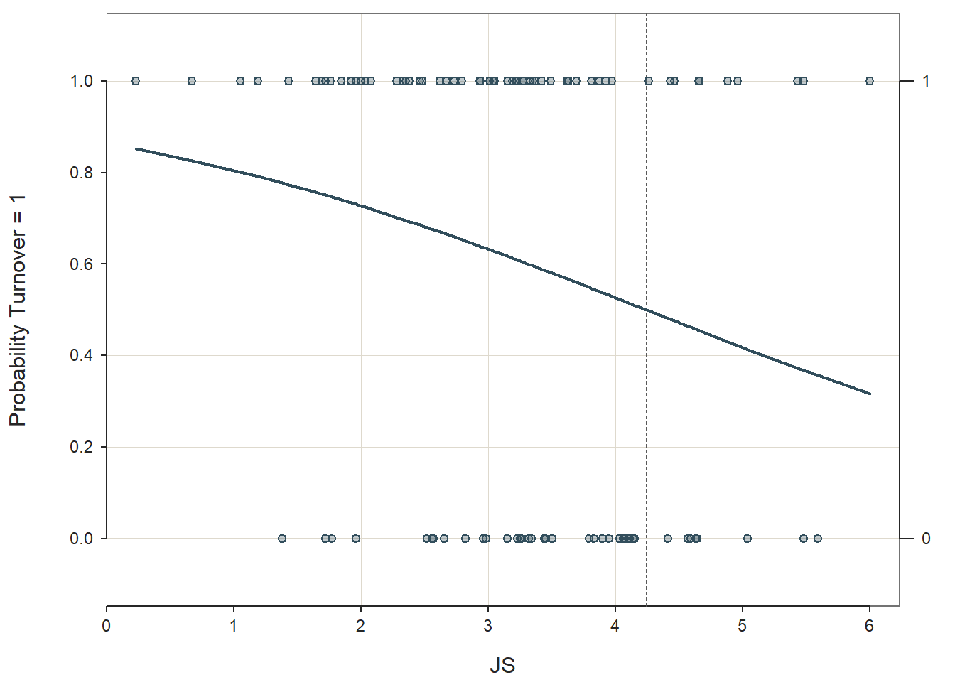
If we print the first six rows from the td data frame object, we will see the new column containing the predicted probabilities based on our simple logistic regression model.
##   Row.names     ID Turnover   JS   OC   TI NAff JS_0 JS_1   prob_JS
## 1         1 EMP559        1 4.96 5.32 0.51 1.87 4.73 5.73 0.4216566
## 2        10 EMP614        1 1.69 2.82 2.58 2.07 1.46 2.46 0.7531576
## 3        11 EMP617        1 3.62 1.08 3.53 2.74 3.39 4.39 0.5672481
## 4        12 EMP619        0 1.72 3.88 1.78 2.11 1.49 2.49 0.7507079
## 5        13 EMP634        0 1.96 3.02 3.41   NA 1.73 2.73 0.7305327
## 6        14 EMP636        0 4.14 2.69 4.33 3.07 3.91 4.91 0.5107466
We can then take those predicted probabilities and apply a threshold by which scores higher than that threshold will indicate that the event is likely to happen. A common threshold for dichotomous outcomes is .50. We’ll use the mutate function from the dplyr package (Wickham et al. 2023) and the ifelse function base R to make this happen.
# Classify probabilities as 1 (Quit) or 0 (Stay)
# Using threshold of .50
td <- mutate(td,
             Pred_Turnover = ifelse(prob_JS >= .50, # apply threshold
                                    1, # if logical statement is true ("Quit")
                                    0) # if logical statement is false ("Stay")
)
It’s important to keep in mind that these predicted probabilities are estimated based on the same data we used to estimate the model in the first place. Given this, I would describe this process as predict-ish analytics as opposed to true predictive analytics. To reach predictive analytics, we would need to obtain “fresh” data on the JS predictor variable, which we could then use to plug into our model; to do this with a model estimated using the Logit model, setting up the model as follows may be the best course of action.
##
## Response Variable:   Turnover
## Predictor Variable 1:  JS
##
## Number of cases (rows) of data:  99
## Number of cases retained for analysis:  98
##
##
##    BASIC ANALYSIS
##
## -- Estimated Model of Turnover for the Logit of Reference Group Membership
##
##              Estimate    Std Err  z-value  p-value   Lower 95%   Upper 95%
## (Intercept)    1.8554     0.6883    2.695    0.007      0.5063      3.2044
##          JS   -0.4378     0.1958   -2.236    0.025     -0.8216     -0.0540
##
##
## -- Odds Ratios and Confidence Intervals
##
##              Odds Ratio   Lower 95%   Upper 95%
## (Intercept)      6.3939      1.6591     24.6415
##          JS      0.6455      0.4397      0.9475
##
##
## -- Model Fit
##
##     Null deviance: 131.746 on 97 degrees of freedom
## Residual deviance: 126.341 on 96 degrees of freedom
##
## AIC: 130.3413
##
## Number of iterations to convergence: 4
##
##
##    ANALYSIS OF RESIDUALS AND INFLUENCE
## Data, Fitted, Residual, Studentized Residual, Dffits, Cook's Distance
##    [sorted by Cook's Distance]
##    [res_rows = 20 out of 98 cases (rows) of data]
## --------------------------------------------------------------------
##      JS Turnover fitted residual rstudent  dffits   cooks
## 66 6.00        1 0.3162   0.6838   1.5688  0.3725 0.08496
## 67 1.38        0 0.7775  -0.7775  -1.7682 -0.2877 0.06241
## 71 5.48        1 0.3673   0.6327   1.4476  0.2949 0.04889
## 54 5.43        1 0.3724   0.6276   1.4363  0.2877 0.04618
## 4  1.72        0 0.7507  -0.7507  -1.6920 -0.2486 0.04353
## 25 1.77        0 0.7466  -0.7466  -1.6810 -0.2429 0.04117
## 5  1.96        0 0.7305  -0.7305  -1.6393 -0.2219 0.03314
## 1  4.96        1 0.4217   0.5783   1.3332  0.2239 0.02609
## 27 4.88        1 0.4302   0.5698   1.3162  0.2138 0.02353
## 83 4.66        1 0.4540   0.5460   1.2703  0.1875 0.01757
## 60 4.65        1 0.4551   0.5449   1.2682  0.1863 0.01733
## 58 2.52        0 0.6797  -0.6797  -1.5199 -0.1668 0.01693
## 97 5.59        0 0.3562  -0.3562  -0.9554 -0.2021 0.01693
## 68 5.48        0 0.3673  -0.3673  -0.9731 -0.1985 0.01648
## 72 2.56        0 0.6758  -0.6758  -1.5115 -0.1635 0.01615
## 73 2.57        0 0.6749  -0.6749  -1.5095 -0.1626 0.01596
## 64 2.65        0 0.6671  -0.6671  -1.4929 -0.1563 0.01454
## 79 5.04        0 0.4131  -0.4131  -1.0457 -0.1813 0.01431
## 75 4.46        1 0.4757   0.5243   1.2296  0.1656 0.01336
## 33 4.43        1 0.4790   0.5210   1.2235  0.1625 0.01282
##
##
##    PREDICTION
##
## Probability threshold for classification : 0.5
##
##
## Data, Fitted Values, Standard Errors
##    [sorted by fitted value]
##    [pred_all=TRUE to see all intervals displayed]
## --------------------------------------------------------------------
##      JS Turnover label fitted std.err
## 66 6.00        1     0 0.3162  0.1215
## 97 5.59        0     0 0.3562  0.1120
## 68 5.48        0     0 0.3673  0.1090
## 71 5.48        1     0 0.3673  0.1090
##
## ... for the rows of data where fitted is close to 0.5 ...
##
##      JS Turnover label fitted std.err
## 33 4.43        1     0 0.4790 0.07497
## 82 4.41        0     0 0.4812 0.07431
## 61 4.26        1     0 0.4976 0.06946
## 20 4.15        0     1 0.5097 0.06609
## 6  4.14        0     1 0.5107 0.06579
##
## ... for the last 4 rows of sorted data ...
##
##      JS Turnover label fitted std.err
## 63 1.19        1     1 0.7916 0.07790
## 43 1.05        1     1 0.8015 0.07904
## 87 0.67        1     1 0.8266 0.08096
## 17 0.23        1     1 0.8525 0.08116
## --------------------------------------------------------------------
##
##
## ----------------------------
## Specified confusion matrices
## ----------------------------
##
## Probability threshold for predicting : 0.5
## Corresponding cutoff threshold for JS: 4.238
##
##                  Baseline         Predicted
## ---------------------------------------------------
##                 Total  %Tot        0      1  %Correct
## ---------------------------------------------------
##            1       59  60.2       10     49     83.1
## Turnover   0       39  39.8        8     31     20.5
## ---------------------------------------------------
##          Total     98                           58.2
##
## Accuracy: 58.16
## Sensitivity: 83.05
## Precision: 61.25
# Extract intercept and predictor coefficient
b0 = unname(mod$coefficients["(Intercept)"]) # extract intercept
b1 = unname(mod$coefficients["JS"]) # extract predictor coefficient

# Specify equation to estimate predicted probabilities
# using sample data on which model was estimated
td$prob_JS_alt <- exp(b0 + b1*td$JS) / (1 + exp(b0 + b1*td$JS))
If we so desired, we could plug in new values for JS from another data frame object like we did in the chapter on predicting criterion scores using simple linear regression. Or we could specify a vector of values for JS that we wish to compute the predicted probabilities of turnover.
# Create vector of plausible values for JS
vec_JS <- c(0,1,2,3,4,5,6)

# "Plug in" vector of values in equation
exp(b0 + b1*vec_JS) / (1 + exp(b0 + b1*vec_JS))
## [1] 0.8647542 0.8049594 0.7270717 0.6322888 0.5260465 0.4173924 0.3162077The 7 predicted probabilities for turning over corresponding to the 7 values we listed in our vector have been printed in order to our Console.
48.2.5 Estimate Multiple Logistic Regression Model
Now we will expand our initial model by specifying a multiple logistic regression model, which means the model will include more than one predictor variable. Let’s begin by regressing Turnover on JS, NAff, and TI using the Logit function from the lessR package. If you haven’t already, install and access the lessR package.
As the first argument in the Logit function, specify the logistic regression model, wherein the dichotomous outcome variable is typed to the left of the ~ symbol, and the predictor variables are typed to the right of the ~ symbol. Separate predictor variables with the + symbol. As the second argument, type data= followed by the name of the data frame to which both of the variables belong (td). Let’s estimate a model with JS, NAff, and TI as the predictor variables.
##
## Response Variable:   Turnover
## Predictor Variable 1:  JS
## Predictor Variable 2:  NAff
## Predictor Variable 3:  TI
##
## Number of cases (rows) of data:  99
## Number of cases retained for analysis:  95
##
##
##    BASIC ANALYSIS
##
## -- Estimated Model of Turnover for the Logit of Reference Group Membership
##
##              Estimate    Std Err  z-value  p-value   Lower 95%   Upper 95%
## (Intercept)   -3.9286     1.8120   -2.168    0.030     -7.4800     -0.3772
##          JS   -0.2332     0.2215   -1.053    0.293     -0.6674      0.2010
##        NAff    1.1952     0.4996    2.392    0.017      0.2160      2.1743
##          TI    0.8967     0.3166    2.832    0.005      0.2761      1.5172
##
##
## -- Odds Ratios and Confidence Intervals
##
##              Odds Ratio   Lower 95%   Upper 95%
## (Intercept)      0.0197      0.0006      0.6858
##          JS      0.7920      0.5130      1.2227
##        NAff      3.3041      1.2411      8.7963
##          TI      2.4514      1.3180      4.5593
##
##
## -- Model Fit
##
##     Null deviance: 127.017 on 94 degrees of freedom
## Residual deviance: 105.229 on 91 degrees of freedom
##
## AIC: 113.2285
##
## Number of iterations to convergence: 4
##
##
## Collinearity
##
##      Tolerance       VIF
## JS       0.885     1.129
## NAff     0.973     1.028
## TI       0.903     1.108
##
##    ANALYSIS OF RESIDUALS AND INFLUENCE
## Data, Fitted, Residual, Studentized Residual, Dffits, Cook's Distance
##    [sorted by Cook's Distance]
##    [res_rows = 20 out of 95 cases (rows) of data]
## --------------------------------------------------------------------
##      JS NAff   TI Turnover  fitted residual rstudent  dffits   cooks
## 6  4.14 3.07 4.33        0 0.93448  -0.9345  -2.4565 -0.4581 0.15185
## 1  4.96 1.87 0.51        1 0.08371   0.9163   2.3396  0.4680 0.13427
## 66 6.00 1.45 2.37        1 0.18699   0.8130   1.9301  0.5252 0.10092
## 42 4.57 2.01 4.27        0 0.77499  -0.7750  -1.8127 -0.5016 0.08228
## 96 2.82 2.05 4.25        0 0.84220  -0.8422  -1.9794 -0.3798 0.05870
## 74 3.50 3.28 1.37        0 0.59961  -0.5996  -1.4140 -0.4473 0.04692
## 27 4.88 1.76 1.81        1 0.20749   0.7925   1.8220  0.3639 0.04554
## 26 3.15 2.84 3.48        0 0.86430  -0.8643  -2.0397 -0.3080 0.04250
## 67 1.38 2.30 3.18        0 0.79411  -0.7941  -1.8204 -0.3391 0.03973
## 61 4.26 1.73 2.10        1 0.27461   0.7254   1.6390  0.3009 0.02635
## 68 5.48 2.27 2.78        0 0.49981  -0.4998  -1.2109 -0.3241 0.02182
## 4  1.72 2.11 1.78        0 0.44724  -0.4472  -1.1203 -0.3091 0.01882
## 25 1.77 2.24 1.16        0 0.34887  -0.3489  -0.9604 -0.3157 0.01803
## 52 3.44 2.35 3.37        0 0.75019  -0.7502  -1.6856 -0.2364 0.01720
## 54 5.43 3.01 2.43        1 0.64141   0.3586   0.9747  0.3071 0.01719
## 69 3.23 2.84 2.18        0 0.66088  -0.6609  -1.4931 -0.2582 0.01719
## 8  3.95 2.87 1.36        0 0.45014  -0.4501  -1.1216 -0.2899 0.01661
## 75 4.46 2.81 1.80        1 0.50095   0.4991   1.2014  0.2785 0.01611
## 77 3.01 1.53 3.01        1 0.47428   0.5257   1.2459  0.2729 0.01593
## 64 2.65 1.94 3.27        0 0.66911  -0.6691  -1.5074 -0.2437 0.01552
##
##
##    PREDICTION
##
## Probability threshold for classification : 0.5
##
##
## Data, Fitted Values, Standard Errors
##    [sorted by fitted value]
##    [pred_all=TRUE to see all intervals displayed]
## --------------------------------------------------------------------
##      JS NAff   TI Turnover label  fitted std.err
## 1  4.96 1.87 0.51        1     0 0.08371 0.05860
## 97 5.59 1.60 1.62        0     0 0.13385 0.07684
## 99 4.06 2.19 0.65        0     0 0.15774 0.08794
## 66 6.00 1.45 2.37        1     0 0.18699 0.10944
##
## ... for the rows of data where fitted is close to 0.5 ...
##
##      JS NAff   TI Turnover label fitted std.err
## 77 3.01 1.53 3.01        1     0 0.4743 0.11354
## 53 3.87 1.72 3.05        1     0 0.4899 0.09955
## 68 5.48 2.27 2.78        0     0 0.4998 0.13673
## 75 4.46 2.81 1.80        1     1 0.5009 0.11987
## 78 3.92 2.80 1.70        1     1 0.5070 0.11250
##
## ... for the last 4 rows of sorted data ...
##
##      JS NAff   TI Turnover label fitted std.err
## 17 0.23 2.38 4.20        1     1 0.9327 0.04890
## 6  4.14 3.07 4.33        0     1 0.9345 0.04905
## 19 2.73 3.64 3.36        1     1 0.9426 0.04146
## 95 2.48 3.18 4.74        1     1 0.9719 0.02322
## --------------------------------------------------------------------
##
##
## ----------------------------
## Specified confusion matrices
## ----------------------------
##
## Probability threshold for predicting : 0.5
##
##                  Baseline         Predicted
## ---------------------------------------------------
##                 Total  %Tot        0      1  %Correct
## ---------------------------------------------------
##            1       58  61.1        6     52     89.7
## Turnover   0       37  38.9       23     14     62.2
## ---------------------------------------------------
##          Total     95                           78.9
##
## Accuracy: 78.95
## Sensitivity: 89.66
## Precision: 78.79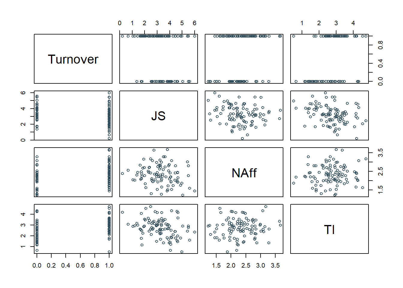
Note: In some instances, you might receive the error message shown below. You can ignore this message, as it just indicates that you have a poor predictor variable in the model that results in fitted/predicted values that are all the same. If you get this message, proceed forward with your interpretation of the output.
\(\color{red}{\text{Error:}}\) \(\color{red}{\text{All predicted values are 0.}}\) \(\color{red}{\text{Something is wrong here.}}\)
The output generates the model coefficient estimates, the odds ratios and confidence intervals, model fit information (i.e., AIC), collinearity diagnostics, outlier detection, forecasts, and a confusion matrix. At the top of the output, we get information about which variables were included in our model, the number of cases (e.g., employees) in the data, and the number of cases retained for the analysis (N = 95) after removing cases with missing data on any of the model variables.
48.2.5.1 Test Statistical Assumptions
To determine whether it’s appropriate to interpret the results of a multiple logistic regression model, we need to first test the following statistical assumptions.
Cases Are Randomly Sampled from the Population: As mentioned in the statistical assumptions section, we will assume that the cases (i.e., employees) were randomly sampled from the population, and thus conclude that this assumption has been satisfied.
Outcome Variable Is Dichotomous: We already know that the outcome variable called Turnover is dichotomous (1 = quit, 0 = stayed), which means we have satisfied this assumption.
Data Are Free of Multivariate Outliers: To determine whether the data are free of multivariate outliers, let’s take a look at the text output section called Analysis of Residuals and Influence. We should find a table with a unique identifiers column (that shows the row number in your data frame object), the observed (actual) predictor and outcome variable values, the fitted (predicted) outcome variable values, the residual (error) between the fitted values and the observed outcome variable values, and the following three outlier/influence statistics: Studentized residual (rstdnt), number of standard error units that a fitted value shifts when the flagged case is removed (dffits), and Cook’s distance (cooks). The case associated with row number 14 has the highest Cook’s distance value (.152), followed by the cases associated with row numbers 1 (.134), 69 (.101), and 47 (.082). A liberal threshold Cook’s distance is 1, which means that we would grow concerned if any of these values exceeded 1, whereas a more conservative threshold is 4 divided by the sample size (4 / 98 = .041). As a sensitivity analysis, we could estimate our model once more after removing the cases associated with row numbers 14, 1, 69 and 47 from our data frame; though, I wouldn’t necessarily recommend this, as these Cook’s distance values aren’t too concerning. In general, we should be wary of removing outliers or influential cases and should do so only when we have a very strong justification for doing so.
No (Multi)Collinearity Between Predictor Variables: To assess whether (multi)collinearity might be an issue, check out the table called Collinearity in the output. This table shows two indices of collinearity: tolerance and valence inflation factor (VIF). Because the VIF is just the reciprocal of the tolerance (1/tolerance), let’s focus just on the tolerance statistic. The tolerance statistic is computed based on the shared variance (R2) of just the predictor variables in a single model (excluding the outcome variable) and subtracting that value from 1 (1 - R2), where a focal predictor variable serves as the outcome and the other(s) (collectively) explain variance in that predictor variable. We typically get concerned when the tolerance statistics approaches .20, as the closer it gets to .00, the higher the collinearity. Ideally, we want the tolerance statistic to approach 1.00, as this indicates that there are very lower levels of collinearity. In the table, we can see that the tolerance statistics are all closer to 1.00 and well above .20, thereby indicating that collinearity is not likely an issue.
Association Between Any Continuous Predictor Variable and Logit Transformation of Outcome Variable Is Linear: To investigate the assumption of linearity between continuous predictor variables and the logit transformation of the outcome variable, we can add the interaction between each continuous predictor variable and its logarithmic (i.e., natural log) transformation. We will use an approach that is commonly referred to as the Box-Tidwell approach (Hosmer and Lemeshow 2000). To apply this approach, we need to add the interaction term between each predictor variable (i.e., JS, NAff, TI) and its logarithmic transformation to our logistic regression model – but not the main effect for the logarithmic transformation. In our regression model formula, specify the dichotomous outcome variable Turnover to the left of the ~ operator. To the right of the ~ operator, type the name of each predictor variable JS followed by the + operator. After the + operator, type the name of the same predictor variable JS, followed by the : operator and the log function from base R with the predictor variable as its sole parenthetical argument. Repeat that process for all continuous predictor variables in the model.
# Box-Tidwell diagnostic test of linearity between continuous predictor variables and
# logit transformation of outcome variable
Logit(Turnover ~ JS + JS:log(JS) + NAff + NAff:log(NAff) + TI + TI:log(TI), data=td)
##
## Response Variable: Turnover
## Predictor Variable 1: JS
## Predictor Variable 2: NAff
## Predictor Variable 3: TI
##
## Number of cases (rows) of data: 99
## Number of cases retained for analysis: 95
##
##
## BASIC ANALYSIS
##
## -- Estimated Model of Turnover for the Logit of Reference Group Membership
##
## Estimate Std Err z-value p-value Lower 95% Upper 95%
## (Intercept) 0.9206 9.8331 0.094 0.925 -18.3519 20.1932
## JS -4.5845 2.6176 -1.751 0.080 -9.7149 0.5459
## NAff -0.4107 6.4047 -0.064 0.949 -12.9636 12.1422
## TI 3.2888 3.0158 1.091 0.275 -2.6221 9.1998
## JS:log(JS) 2.0053 1.1844 1.693 0.090 -0.3160 4.3266
## NAff:log(NAff) 0.9559 3.5321 0.271 0.787 -5.9670 7.8788
## TI:log(TI) -1.2101 1.5232 -0.794 0.427 -4.1956 1.7754
##
##
## -- Odds Ratios and Confidence Intervals
##
## Odds Ratio Lower 95% Upper 95%
## (Intercept) 2.5108 0.0000 588545072.9794
## JS 0.0102 0.0001 1.7261
## NAff 0.6632 0.0000 187626.1824
## TI 26.8110 0.0726 9894.6983
## JS:log(JS) 7.4284 0.7291 75.6872
## NAff:log(NAff) 2.6010 0.0026 2640.6975
## TI:log(TI) 0.2982 0.0151 5.9024
##
##
## -- Model Fit
##
## Null deviance: 127.017 on 94 degrees of freedom
## Residual deviance: 100.854 on 88 degrees of freedom
##
## AIC: 114.8541
##
## Number of iterations to convergence: 5
##
##
## Collinearity
##
## Tolerance VIF
## JS 0.030 32.947
## NAff 0.012 82.947
## TI 0.073 13.775
##
## ANALYSIS OF RESIDUALS AND INFLUENCE
## Data, Fitted, Residual, Studentized Residual, Dffits, Cook's Distance
## [sorted by Cook's Distance]
## [res_rows = 20 out of 95 cases (rows) of data]
## --------------------------------------------------------------------
## JS NAff TI Turnover fitted residual rstudent dffits cooks
## 1 4.96 1.87 0.51 1 0.03086 0.9691 3.2985 0.9563 0.63056
## 6 4.14 3.07 4.33 0 0.91111 -0.9111 -2.3981 -0.6526 0.14155
## 67 1.38 2.30 3.18 0 0.91516 -0.9152 -2.3760 -0.5617 0.10829
## 68 5.48 2.27 2.78 0 0.73899 -0.7390 -1.7745 -0.6741 0.07686
## 66 6.00 1.45 2.37 1 0.55250 0.4475 1.2378 0.7960 0.07043
## 42 4.57 2.01 4.27 0 0.72166 -0.7217 -1.7245 -0.6507 0.06898
## 74 3.50 3.28 1.37 0 0.50709 -0.5071 -1.3129 -0.6965 0.05735
## 96 2.82 2.05 4.25 0 0.72223 -0.7222 -1.6950 -0.5521 0.04977
## 79 5.04 1.22 2.92 0 0.42774 -0.4277 -1.1658 -0.6487 0.04597
## 4 1.72 2.11 1.78 0 0.53924 -0.5392 -1.3118 -0.4774 0.02800
## 27 4.88 1.76 1.81 1 0.25761 0.7424 1.6982 0.3893 0.02590
## 25 1.77 2.24 1.16 0 0.31999 -0.3200 -0.9531 -0.5030 0.02531
## 26 3.15 2.84 3.48 0 0.83033 -0.8303 -1.9278 -0.3366 0.02494
## 81 3.34 1.27 2.96 0 0.33222 -0.3322 -0.9633 -0.4596 0.02133
## 77 3.01 1.53 3.01 1 0.41376 0.5862 1.3781 0.4014 0.02101
## 21 3.37 1.65 4.16 1 0.57404 0.4260 1.1068 0.4163 0.01894
## 61 4.26 1.73 2.10 1 0.26659 0.7334 1.6620 0.3239 0.01759
## 70 2.08 1.62 4.55 1 0.75821 0.2418 0.7970 0.3930 0.01463
## 52 3.44 2.35 3.37 0 0.68034 -0.6803 -1.5371 -0.2832 0.01210
## 58 2.52 1.30 2.13 0 0.24723 -0.2472 -0.7985 -0.3562 0.01207
##
##
## PREDICTION
##
## Probability threshold for classification : 0.5
##
##
## Data, Fitted Values, Standard Errors
## [sorted by fitted value]
## [pred_all=TRUE to see all intervals displayed]
## --------------------------------------------------------------------
## JS NAff TI Turnover label fitted std.err
## 1 4.96 1.87 0.51 1 0 0.03086 0.05764
## 99 4.06 2.19 0.65 0 0 0.04451 0.06863
## 88 4.07 2.21 1.21 0 0 0.14009 0.09587
## 46 3.79 1.45 1.83 0 0 0.15073 0.09141
##
## ... for the rows of data where fitted is close to 0.5 ...
##
## JS NAff TI Turnover label fitted std.err
## 49 4.63 2.45 2.01 0 0 0.4820 0.1237
## 86 3.42 2.23 2.57 1 0 0.4962 0.1032
## 28 2.67 1.95 2.68 1 0 0.4997 0.1070
## 74 3.50 3.28 1.37 0 1 0.5071 0.2402
## 13 2.98 2.32 2.41 0 1 0.5145 0.1018
##
## ... for the last 4 rows of sorted data ...
##
## JS NAff TI Turnover label fitted std.err
## 95 2.48 3.18 4.74 1 1 0.9499 0.063267
## 19 2.73 3.64 3.36 1 1 0.9537 0.060780
## 87 0.67 2.56 3.08 1 1 0.9890 0.020304
## 17 0.23 2.38 4.20 1 1 0.9988 0.003638
## --------------------------------------------------------------------
##
##
## ----------------------------
## Specified confusion matrices
## ----------------------------
##
## Probability threshold for predicting : 0.5
##
## Baseline Predicted
## ---------------------------------------------------
## Total %Tot 0 1 %Correct
## ---------------------------------------------------
## 1 58 61.1 8 50 86.2
## Turnover 0 37 38.9 21 16 56.8
## ---------------------------------------------------
## Total 95 74.7
##
## Accuracy: 74.74
## Sensitivity: 86.21
## Precision: 75.76
Because the p-values associated with each of the interaction terms and their regression coefficients (JS:log(JS), NAff:log(NAff), TI:log(TI)) are equal to or greater than the conventional two-tailed alpha level of .05, we have no reason to believe that any of the associations between the continuous predictor variables and the logit transformation of the outcome variable are nonlinear. If one of the interaction terms had been statistically significant, then we might have evidence that the assumption was violated, meaning we would assume a nonlinear association instead, and one potential solution would be to apply a transformation to the predictor variable in question (e.g., logarithmic transformation). Finally, we only apply this test when the predictor variables in question are continuous (interval, ratio).
Important Note: If the variable for which you are applying the Box-Tidwell approach described above has one or more cases with a score of zero, then you will receive an error message when you run the model with the log function. The reason for the error is that the log of zero or any negative value is (mathematically) undefined. There are many reasons why your variable might have cases with scores equal to zero, some of which include: (a) zero is a naturally occurring value for the scale on which the variable is based, or (b) the variable was grand-mean centered or standardized, such that the mean is now equal to zero. There are some approaches to dealing with this issue and neither approach I will show you is going to be perfect, but each approach will give you an approximate understanding of whether violation of the linearity assumption might be an issue. First, we can add a positive numeric constant to every score on the continuous predictor variable in question that will result in the new lowest score being 1. Why 1 you might ask? Well, the rationale is somewhat arbitrary; the log of 1 is zero, and there is something nice about grounding the lowest logarithmic value at 0. Due note, however, that the magnitude of the linear transformation will have some effect on the p-value associated with the Box-Tidwell interaction term. Second, if there are proportionally very few cases with scores of zero on the predictor variable in question, we can simply subset those cases out for the analysis. These approaches to addressing zero values (including the error message you might encounter) are demonstrated in a previous section on simple logistic regression.
48.2.5.2 Interpret Model Results
Basic Analysis: The Basic Analysis section of the original output first displays a table called the Model Coefficients, which includes the regression coefficients (slopes, weights) and their standard errors, z-values, p-values, and lower and upper limits of their 95% confidence intervals. Typically, the intercept value and its significance test are not of interest, unless we wish to use the value to specify the regression model equation. The estimate of the unstandardized regression coefficient for the predictor variable (JS) in relation to the logit transformation of the outcome variable (Turnover) is not statistically significant when controlling for the other predictor variables in the model because the associated p-value is equal to or greater than .05 (b = -.233, p = .293, 95% CI[-0.667, .201]). The regression coefficient for NAff is 1.195 and its associated p-value is less than .05, indicating that the association is statistically significant when controlling for the other predictor variables in the model (b = 1.195, p = .017, 95% CI[.216, 2.174]). Finally, the regression coefficient for TI is .897 and its associated p-value is less than .05, indicating that the association is also statistically significant when controlling for the other predictor variables in the model (b = .897, p = .005, 95% CI[.276, 1.517]).
Given that one of the predictor variables did not share a statistically significant association with the outcome when included in the model, in some contexts we might not write out the regression equation with that variable included; instead, we might re-estimate the model without that variable. For illustrative purposes, however, we will write out the equation. Using the intercept and predictor variable coefficient estimates, we can write out the equation for the regression model as follows:
\(\ln(\frac{p}{1-p}) = -3.929 - .233 \times JS_{observed} + 1.195 \times NAff_{observed} + .897 \times TI_{observed}\)
where \(p\) refers to, in this example, as the probability of quitting. If you recall from earlier in the tutorial, we can also interpret our findings with respect to \(\log(odds)\).
\(\log(odds) = \ln(\frac{p}{1-p}) = -3.929 - .233 \times JS_{observed} + 1.195 \times NAff_{observed} + .897 \times TI_{observed}\)
To that end, to aid our interpretation of the significant finding, we can move our attention to the table called Odds ratios and confidence intervals. To convert our regression coefficients to odds ratios, the function is simply exponentiating them. Behind the scenes, this is what happened:
\(e^{1.195} = 3.304\)
We can also do this manually using the exp function from base R. Any difference between the Logit output and the output below is attributable to rounding.
# For the sake of demonstration:
# Exponentiate logistic regression coefficient to convert to odds ratio
# Note that the Logit function already does this for us
exp(1.195)
## [1] 3.303558In the Odds ratios and confidence intervals table, we see that the odds ratios are automatically computed for us. We should only interpret those odds ratios in which their corresponding regression coefficient was statistically significant; accordingly, in this example, we will just interpret the odds ratios belong to NAff and TI. Regarding NAff, its odds ratio of 3.304 is greater than 1, which implies a positive association between the predictor and the outcome variables, which we already knew from the negative regression coefficient on which it is based. Thus, the odds of quitting are 3.304 times greater for every one unit increase in NAff when controlling for other predictor variables in the model. Regarding TI, its odds ratio of 2.451 is also greater than 1, and thus, the odds of quitting are 2.451 times greater for every one unit increase in TI when controlling for other predictor variables in the model. Note that the odds ratio (OR) can be conceptualized as a type of effect size, and thus we can compare odds ratios and describe an odds ratio qualitatively using descriptive language. There are different rules of thumb, and for the sake of parsimony, I provide rules of thumb for when odds ratios are greater than 1 and less than 1. Both odds ratios are about medium in terms of their magnitude.
| Odds Ratio > 1 | Odds Ratio < 1 | Description |
|---|---|---|
| 1.2 | .8 | Small |
| 2.5 | .4 | Medium |
| 4.3 | .2 | Large |
In the Model Fit table, note that we don’t have an estimate of R-squared (R2) like we would with a traditional linear regression model. There are ways to compute what are often referred to as pseudo-R-squared (R2) values, but for now let’s focus on what is produced in the Logit function output. As you can see, we get the null deviance and residual deviance values (and their degrees of freedom) as well as the Akaike information criterion (AIC) value. By themselves, these values are not very meaningful; however, they can be used to compare nested models, which is beyond the scope of this tutorial. For our purposes, we will assess the model’s fit to the data by looking at the Specified Confusion Matrices table at the end of the output. This table makes model fit assessments fairly intuitive. First, in the baseline section (which is akin to a null model without any predictors), the confusion matrix provides information about actual the counts and percentages of employees who stayed and quit the organization, which were 37 (38.9%) and 58 (61.1%), respectively. [Remember that for the Turnover variable, 0 = stayed and 1 = quit in our data.] In the predicted section, the table provides information about who would be predicted to stay and who would be predicted to quit based on our logistic regression model. Anyone who has a predicted probability of .50 or higher is predicted to quit, and anyone who has a predicted probability that is less than .50 is predicted to stay. Further, a cross-tabulation is shown in which the rows represent actual/observed turnover behavior (0 = stay, 1 = quit), and the columns represent predicted turnover behavior (0 = stay, 1 = quit). Thus, this cross-tabulation helps us understand how accurate our model predictions were relative to the observed data, thereby providing us with an indication of how well the model fit the data. Of those who actually stayed (0), we were able to predict their turnover behavior with 62.2% accuracy using our model. Of those who actually quit (1), our model fared much better, as we were able to predict that outcome with 89.7% accuracy. Overall, we tend to be most interested in the overall percentage of correct classifications, which is 78.9%. That is, based on the logistic regression model that included the predictor variables of JS, NAff, and TI, we were able to predict actual turnover behavior from the same sample 78.9% of the time, which was a big improvement over the simple logistic regression model in which we had just JS as a predictor variable.
Forecasts: In the output section called Forecasts, information about the actual outcome and the predicted and fitted values are presented (along with the standard error). This section moves us toward what would be considered true predictive analytics and machine learning; however, because we only have a single dataset to train our model and test it, we’re not performing true predictive analytics. As such, we won’t pay much attention to interpreting this section of the output in this tutorial. With that said, if you’re curious, feel free to read on. When performing true predictive analytics, we typically divide our data into at least two datasets. Often, we have at least one training dataset that we use to “train” or estimate a given model; often, we have more than one training dataset, though. After training the model on one or more training datasets, we then evaluate the model on a test dataset that should contain data from an entirely different set of cases than the training dataset(s). As a more rigorous approach, we can instead use a validation dataset to evaluate the training dataset(s), and after we’ve picked the model that performs best on the validation set, we then pass the model along to the test dataset to see if we can confirm the results.
Nagelkerke pseudo-R2: To compute Nagelkerke’s pseudo-R2, we will need to install and access the DescTools package (if we haven’t already) so that we can use its PseudoR2 function.
To use the function, we’ll need to re-estimate our multiple logistic regression model using the glm function from base R. To request a logistic regression model as a specific type of generalized linear model, we’ll add the family=binomial argument. Using the <- assignment operator, we will assign the resulting estimated model to an object that we’ll arbitrarily call model2.
# Estimate simple logistic regression model and assign to object
model2 <- glm(Turnover ~ JS + NAff + TI, data=td, family=binomial)
In the PseudoR2 function, we will specify the name of the model object (model2) as the first argument. As the second argument, type "Nagel" to request pseudo-R2 calculated using Nagelkerke’s formula.
## Nagelkerke
##  0.2779516
The estimated Nagelkerke pseudo-R2 is .278, which is a big improvement over the simple logistic regression model we estimated above for which pseudo-R2 was just .073. Remember, a pseudo-R2 is not the exact same thing as a true R2, so we should interpret it with caution. With caution, we can conclude that JS, NAff, and TI explain 27.8% of the variance in Turnover.
Because the DescTools package also has a function called Logit, let’s detach the package before moving forward so that we don’t inadvertently attempt to use the Logit function from DescTools as opposed to the one from lessR.
Technical Write-Up of Results: A turnover study was conducted based on a sample of 99 employees from the past year, some of whom quit the company and some of whom stayed. Turnover behavior (quit vs. stay) (Turnover) is our outcome of interest, and because it is dichotomous, we used logistic regression. We, specifically, were interested in the extent to which employees’ self-reported job satisfaction, negative affectivity, and turnover intentions were associated with their decisions to quit or stay, and thus all three were was used as continuous predictor variables in our multiple logistic regression model. In total, due to missing data, 95 employees were included in our analysis. Results indicated that, indeed, job satisfaction was not associated with turnover behavior to a statistically significant extent (b = -.233, p = .293, 95% CI[-0.667, .201]). Negative affectivity, however, was positively and significantly associated with turnover behavior (b = 1.195, p = .017, 95% CI[.216, 2.174]), such that the odds of quitting were 3.304 times as likely for every one unit increase in negative affectivity, when controlling for other predictor variables in the model. Similarly, turnover intentions were also positively and significantly associated with turnover behavior (b = .897, p = .005, 95% CI[.276, 1.517]), such that the odds of quitting were 2.451 times as likely for every one unit increase in turnover intentions, when controlling for other predictor variables in the model. Both of these significant associations were medium in magnitude. Overall, based on our estimated multiple logistic regression model, we were able to predict actual turnover behavior in our sample with 78.9% accuracy. Finally, the estimated Nagelkerke pseudo-R2 was .278. We can cautiously conclude that job satisfaction, negative affectivity, and turnover intentions explain 27.8% of the variance in voluntary turnover.
48.3 Chapter Supplement
In addition to the Logit function from the lessR package covered above, we can use the glm function from base R to estimate a simple and multiple logistic regression models and the predict function from base R to predict probabilities of the event in question occurring. Because these functions come from base R, we do not need to install and access an additional package.
48.3.1 Functions & Packages Introduced
| Function | Package |
|---|---|
glm |
base R |
log |
base R |
exp |
base R |
plot |
base R |
cooks.distance |
base R |
summary |
base R |
confint |
base R / MASS |
coef |
base R |
subset |
base R |
na.omit |
base R |
xtabs |
base R |
print |
base R |
prop.table |
base R |
predict |
base R |
sum |
base R |
scale |
base R |
vif |
car |
PseudoR2 |
DescTools |
c |
base R |
merge |
base R |
data.frame |
base R |
mutate |
dplyr |
ifelse |
base R |
48.3.2 Initial Steps
If required, please refer to the Initial Steps section from this chapter for more information on these initial steps.
# Install readr package if you haven't already
# [Note: You don't need to install a package every
# time you wish to access it]
install.packages("readr")
# Access readr package
library(readr)
# Read data and name data frame (tibble) object
td <- read_csv("Turnover.csv")## Rows: 99 Columns: 6
## ── Column specification ────────────────────────────────────────────────────────────────────────────────────────────────────────────
## Delimiter: ","
## chr (1): ID
## dbl (5): Turnover, JS, OC, TI, NAff
##
## ℹ Use `spec()` to retrieve the full column specification for this data.
## ℹ Specify the column types or set `show_col_types = FALSE` to quiet this message.## [1] "ID" "Turnover" "JS" "OC" "TI" "NAff"## spc_tbl_ [99 × 6] (S3: spec_tbl_df/tbl_df/tbl/data.frame)
## $ ID : chr [1:99] "EMP559" "EMP561" "EMP571" "EMP589" ...
## $ Turnover: num [1:99] 1 1 1 1 1 1 0 1 1 1 ...
## $ JS : num [1:99] 4.96 1.72 1.64 3.01 3.04 3.81 1.38 3.92 2.35 1.69 ...
## $ OC : num [1:99] 5.32 1.47 0.87 2.15 1.94 3.81 0.83 3.88 3.03 2.82 ...
## $ TI : num [1:99] 0.51 4.08 2.65 4.17 3.27 3.01 3.18 1.7 2.44 2.58 ...
## $ NAff : num [1:99] 1.87 2.48 2.84 2.43 2.76 3.67 2.3 2.8 2.71 2.07 ...
## - attr(*, "spec")=
## .. cols(
## .. ID = col_character(),
## .. Turnover = col_double(),
## .. JS = col_double(),
## .. OC = col_double(),
## .. TI = col_double(),
## .. NAff = col_double()
## .. )
## - attr(*, "problems")=<externalptr>## # A tibble: 6 × 6
## ID Turnover JS OC TI NAff
## <chr> <dbl> <dbl> <dbl> <dbl> <dbl>
## 1 EMP559 1 4.96 5.32 0.51 1.87
## 2 EMP561 1 1.72 1.47 4.08 2.48
## 3 EMP571 1 1.64 0.87 2.65 2.84
## 4 EMP589 1 3.01 2.15 4.17 2.43
## 5 EMP592 1 3.04 1.94 3.27 2.76
## 6 EMP601 1 3.81 3.81 3.01 3.6748.3.3 Simple Logistic Regression Model Using glm Function from Base R
The glm function from base R stands for “generalized linear model (GLM),” making it an appropriate function for estimating logistic regression models and other models in the GLM family; logistic regression model is a GLM with a logit link function. Let’s begin by specifying JS as a predictor variable for Turnover.
- Using the
<-assignment operator, we will come up with a name of an object to which we will assign the estimated model (e.g.,model1). - Type the name of the
glmfunction.
- As the function’s first argument, specify the logistic regression model, wherein the dichotomous outcome variable is typed to the left of the
~symbol, and the predictor variable is typed to the right of the~symbol. - As the second argument, type
data=followed by the name of the data frame (td) to which both of the variables belong. - As the third argument, type
family=binomial, which by default estimates a logit (logistic) model.
Note: You won’t see a summary of the results in the Console, as we have not requested those. As a next step, we will use the model1 object to determine whether we have satisfied the statistical assumptions of a simple logistic regression model.
48.3.3.1 Test Statistical Assumptions
To determine whether it’s appropriate to interpret the results of a simple logistic regression model, we need to first test the following statistical assumptions.
Cases Are Randomly Sampled from the Population: As mentioned in the statistical assumptions section, we will assume that the cases (i.e., employees) were randomly sampled from the population, and thus conclude that this assumption has been satisfied.
Outcome Variable Is Dichotomous: We already know that the outcome variable called Turnover is dichotomous (1 = quit, 0 = stayed), which means we have satisfied this assumption.
Data Are Free of Bivariate Outliers: To determine whether the data are free of bivariate outliers, let’s look at Cook’s distance (D) values across cases. Using the plot function from base R, type the name of our model object (model1) as the first argument, and as the second argument, enter the numeral 4 to request the fourth diagnostic plot, which is the Cook’s distance plot.
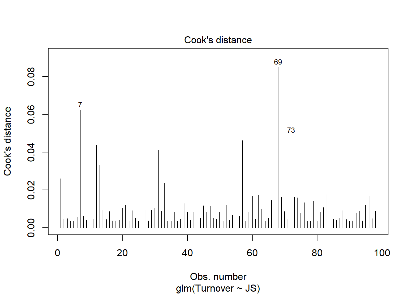
The case associated with row number 66 has the highest Cook’s distance value, followed by the cases associated with row numbers 67 and 71 – although 66 and 67 seem to be clearest potential outliers of the three.
We can also print the cases with the highest Cook’s distances. To do so, let’s create an object called cooksD to which we will assign a vector of Cook’s distance values using the cooks.distance function from base R. Just type the name of the logistic regression model object (model1) as the sole parenthetical argument. Next, update the object we called cooksD by applying the sort function from base R and typing the cooksD object name as the first object and decreasing=TRUE as the second argument; this will sort the Cook’s distance values in descending order. Finally, apply the head function from base R, and as the first argument enter the name of the cooksD object that we just sorted; as the second argument, type n=20 to show the top 20 rows, as opposed to the default top 6 rows.
# Estimate Cook's distance values
cooksD <- cooks.distance(model1)
# Sort Cook's distance values in descending order
cooksD <- sort(cooksD, decreasing=TRUE)
# View top 20 Cook's distance values
head(cooksD, n=20)## 69 7 73 58 12 31 13 1 33 84 63 61
## 0.08495602 0.06240864 0.04888996 0.04617863 0.04352935 0.04117397 0.03313842 0.02608930 0.02352896 0.01756755 0.01733141 0.01693066
## 97 70 74 75 67 80 77 39
## 0.01692984 0.01648318 0.01614505 0.01595550 0.01453516 0.01431210 0.01336026 0.01281733Again, we see cases associated with row numbers 66 (.085), 67 (.062), and 71 (.049) having the highest Cook’s distance values, with 66 and 67 still looking like the most influential cases of the lot. As a sensitivity analysis, we could estimate our model once more after removing the cases associated with row numbers 66 and 67 from our data frame. With that being said, we should be wary of removing outlier or influential cases and should do so only when we have good justification for doing so. A liberal threshold Cook’s distance is 1, which means that we would grow concerned if any of these values exceeded 1, whereas a more conservative threshold is 4 divided by the sample size (4 / 98 = .041). These Cook’s distance values are all well-below the more liberal threshold, so I would say we’re safe to leave the associated cases in the data.
Association Between Any Continuous Predictor Variable and Logit Transformation of Outcome Variable Is Linear: To test the assumption of linearity between a continuous predictor variable and the logit transformation of the outcome variable, we can add the interaction between the predictor variable and its logarithmic (i.e., natural log) transformation. [Note: We do not perform the following test/approach for categorical predictor variables.] We will use an approach that is commonly referred to as the Box-Tidwell approach (Hosmer and Lemeshow 2000). To apply this approach, we need to add the interaction term between our predictor variable JS and its logarithmic transformation to our logistic regression model – but not the main effect for the logarithmic transformation of JS. In our regression model formula, specify the dichotomous outcome variable Turnover to the left of the ~ operator. To the right of the ~ operator, type the name of the predictor variable JS followed by the + operator. After the + operator, type the name of the predictor variable JS, followed by the : operator and the log function from base R with the predictor variable JS as its sole parenthetical argument. Finally, we will use the summary function from base R to generate the model output, and within the parentheses, enter the name of the model you created in the prior step (boxtidwell).
# Box-Tidwell diagnostic test of linearity between continuous predictor variable and
# logit transformation of outcome variable
boxtidwell <- glm(Turnover ~ JS + JS:log(JS), data=td, family=binomial)
# Print summary of results
summary(boxtidwell)##
## Call:
## glm(formula = Turnover ~ JS + JS:log(JS), family = binomial,
## data = td)
##
## Coefficients:
## Estimate Std. Error z value Pr(>|z|)
## (Intercept) 5.4461 3.2062 1.699 0.0894 .
## JS -2.9840 2.1693 -1.376 0.1690
## JS:log(JS) 1.1696 0.9778 1.196 0.2316
## ---
## Signif. codes: 0 '***' 0.001 '**' 0.01 '*' 0.05 '.' 0.1 ' ' 1
##
## (Dispersion parameter for binomial family taken to be 1)
##
## Null deviance: 131.75 on 97 degrees of freedom
## Residual deviance: 124.62 on 95 degrees of freedom
## (1 observation deleted due to missingness)
## AIC: 130.62
##
## Number of Fisher Scoring iterations: 5Because the interaction term (JS:log(JS)) regression coefficient of 1.1696 in the Coefficients table is nonsignificant (p = .232), we have no reason to believe that the association between the continuous predictor variable and the logit transformation of the outcome variable is nonlinear. If the interaction term had been statistically significant, then we might have evidence that the assumption was violated, and one potential solution would be to estimate a polynomial model of some kind to better fit the data; for more information on estimating nonlinear associations, check out Chapter 7 (“Curvilinear Effects in Logistic Regression”) from Osborne (2015). Finally, we only apply this test when the predictor variable in question is continuous (interval, ratio). In practice, however, note that for reasons of parsimony, we sometimes we might choose to estimate a linear model over a nonlinear/polynomial model when the former fits the data reasonably well.
Important Note: If the variable for which you are applying the Box-Tidwell approach described above has one or more cases with a score of zero, then you will receive an error message when you run the model with the log function. The reason for the error is that the log of zero or any negative value is (mathematically) undefined. There are many reasons why your variable might have cases with scores equal to zero, some of which include: (a) zero is a naturally occurring value for the scale on which the variable is based, or (b) the variable was grand-mean centered or standardized, such that the mean is now equal to zero. There are some approaches to dealing with this issue and neither approach I will show you is going to be perfect, but each approach will give you an approximate understanding of whether violation of the linearity assumption might be an issue. First, we can add a positive numeric constant to every score on the continuous predictor variable in question that will result in the new lowest score being 1. Why 1 you might ask? Well, the rationale is somewhat arbitrary; the log of 1 is zero, and there is something nice about grounding the lowest logarithmic value at 0. Due note, however, that the magnitude of the linear transformation will have some effect on the p-value associated with the Box-Tidwell interaction term. Second, if there are proportionally very few cases with scores of zero on the predictor variable in question, we can simply subset those cases out for the analysis.
Just for the sake of demonstration, let’s transform the JS variable so that its lowest score is equal to zero. This will give us an opportunity to test the two approaches I described above. Simply, create a new variable (JS_0) that is equal to JS minus the minimum value of JS.
# ONLY FOR DEMONSTRATION PURPOSES: Create new predictor variable where lowest score is zero
td$JS_0 <- td$JS - min(td$JS, na.rm=TRUE)Now that we have a variable called JS_0 with at least one score equal to zero, let’s try the try the Box-Tidwell test. I’m going to add the argument brief=TRUE to reduce the amount of output generated by the function.
# Box-Tidwell diagnostic test of linearity between continuous predictor variable and
# logit transformation of outcome variable [with predictor containing zero value(s)]
boxtidwell <- glm(Turnover ~ JS_0 + JS_0:log(JS_0), data=td, family=binomial)
# Print summary of results
summary(boxtidwell)If you ran the script above, you likely got an error message that looked like this:
\(\color{red}{\text{Error in glm.fit(x = c(1, 1, 1, 1, 1, 1, 1, 1, 1, 1, 1, 1, 1, 1, 1, 1, : NA/NaN/Inf in 'x'}}\)
The reason we got this error message is because the log of zero is undefined, and because we had at least one case with a value of zero on JS_0, it broke down the operations. If you see a message like that, then proceed with one or both of the following approaches (which I described above).
Using the first approach, create a new variable in which the JS_0 variable is linearly transformed such that the lowest score is 1. The equation below simply adds 1 and the absolute value of the minimum value to each score on the JS_0 variable, which results in the lowest score on the new variable (JS_1) being 1. As verification, I include the min function from base R.
# Linear transformation that results in lowest score being 1
td$JS_1 <- td$JS_0 + abs(min(td$JS_0, na.rm=TRUE)) + 1
# Verify that new lowest score is 1
min(td$JS_1, na.rm=TRUE)## [1] 1It worked! Now, using this new transformed variable, enter it into the Box-Tidwell test.
# Box-Tidwell diagnostic test of linearity between continuous predictor variable and
# logit transformation of outcome variable [with transformed predictor = 1]
boxtidwell <- glm(Turnover ~ JS_1 + JS_1:log(JS_1), data=td, family=binomial)
# Print summary of results
summary(boxtidwell)##
## Call:
## glm(formula = Turnover ~ JS_1 + JS_1:log(JS_1), family = binomial,
## data = td)
##
## Coefficients:
## Estimate Std. Error z value Pr(>|z|)
## (Intercept) 8.099 5.008 1.617 0.106
## JS_1 -4.059 2.977 -1.363 0.173
## JS_1:log(JS_1) 1.510 1.226 1.231 0.218
##
## (Dispersion parameter for binomial family taken to be 1)
##
## Null deviance: 131.75 on 97 degrees of freedom
## Residual deviance: 124.57 on 95 degrees of freedom
## (1 observation deleted due to missingness)
## AIC: 130.57
##
## Number of Fisher Scoring iterations: 4There is no error message this time, and now we can see that the interaction term between the predictor variable and the log of the predictor variable (JS_1:log(JS_1)) is nonsignificant (b = 1.510, p = .218). Thus, we don’t see evidence that the assumption of linearity has been violated.
We could (also) use the second approach if we have proportionally very few values that are zero (or less than zero). To do so, we would just use the rows= argument to specify that we want to drop cases for which the predictor variable is equal to or less than zero. Note that we’re back to using the variable called JS_0 that forced to have at least one score equal to zero (solely for the purposes of demonstration in this tutorial).
# Box-Tidwell diagnostic test of linearity between continuous predictor variable and
# logit transformation of outcome variable [with only cases with scores greater than zero]
boxtidwell <- glm(Turnover ~ JS_0 + JS_0:log(JS_0), data=td, family=binomial, subset=(JS_0 > 0))
# Print summary of results
summary(boxtidwell)##
## Call:
## glm(formula = Turnover ~ JS_0 + JS_0:log(JS_0), family = binomial,
## data = td, subset = (JS_0 > 0))
##
## Coefficients:
## Estimate Std. Error z value Pr(>|z|)
## (Intercept) 4.665 2.822 1.653 0.0982 .
## JS_0 -2.616 1.994 -1.312 0.1895
## JS_0:log(JS_0) 1.039 0.928 1.120 0.2628
## ---
## Signif. codes: 0 '***' 0.001 '**' 0.01 '*' 0.05 '.' 0.1 ' ' 1
##
## (Dispersion parameter for binomial family taken to be 1)
##
## Null deviance: 130.72 on 96 degrees of freedom
## Residual deviance: 124.62 on 94 degrees of freedom
## (1 observation deleted due to missingness)
## AIC: 130.62
##
## Number of Fisher Scoring iterations: 4We lost one case because that person had a score of zero on the JS_0 continuous predictor variable, and we see that the interaction term (JS_0:log(JS_0)) is non significant (b = 1.039, p = .263).
To summarize, the two approaches we just implemented would only be used when testing the statistical assumption of linearity using the Box-Tidwell approach, and only if your continuous predictor variable has scores that are equal to or less than zero. Now that we’ve met the assumption of linearity, we’re finally ready to interpret the model results!
48.3.3.2 Interpret Model Results
Now we’re ready to interpret the results of the simple logistic regression model. For clarity, let’s re-specify our original simple logistic regression model from above. To apply the glm function, type the name of the function. As the first argument, specify the logistic regression model, wherein the dichotomous outcome variable is typed to the left of the ~ symbol, and the predictor variable is typed to the right of the ~ symbol. As the second argument, type data= followed by the name of the data frame (td) to which both of the variables belong. Third, type the argument family=binomial, which by default estimates a logit (logistic) model. Be sure to name and create an object based on your model using the <- assignment operator; here, I again arbitrarily named the object model1. Finally, use the summary function from base R to generate the model output, and within the parentheses, enter the name of the model you created in the prior step (model1).
# Estimate simple logistic regression model
model1 <- glm(Turnover ~ JS, data=td, family=binomial)
# Print summary of results
summary(model1)##
## Call:
## glm(formula = Turnover ~ JS, family = binomial, data = td)
##
## Coefficients:
## Estimate Std. Error z value Pr(>|z|)
## (Intercept) 1.8554 0.6883 2.695 0.00703 **
## JS -0.4378 0.1958 -2.236 0.02538 *
## ---
## Signif. codes: 0 '***' 0.001 '**' 0.01 '*' 0.05 '.' 0.1 ' ' 1
##
## (Dispersion parameter for binomial family taken to be 1)
##
## Null deviance: 131.75 on 97 degrees of freedom
## Residual deviance: 126.34 on 96 degrees of freedom
## (1 observation deleted due to missingness)
## AIC: 130.34
##
## Number of Fisher Scoring iterations: 4The output generates the model coefficient estimates and model fit (i.e., AIC) information.
Coefficients: The Coefficients section of the output displays the regression coefficients (slopes, weights) and their standard errors, z-values, and p-values. Typically, the intercept value and its significance test are not of interest, unless we wish to use the value to specify the regression model equation. The estimate of the regression coefficient for the predictor variable (JS) in relation to the outcome variable (Turnover) is often of substantive interest. Here, we see that the unstandardized regression coefficient for JS is -.438, and its associated p-value is less than .05 (b = -.438, p = .025). Given that the p-value is less than our conventional two-tailed alpha level of .05, we reject the null hypothesis that the regression coefficient is equal to zero, which means that we conclude that the regression coefficient is statistically significantly different from zero. The conceptual interpretation of logistic regression coefficients is not as straightforward as traditional linear regression coefficients, though. We can, however, interpret the significant regression coefficient as follows: For every one unit increase in the predictor variable (JS), the logit transformation of the outcome variable (Turnover) decreases by .438 units. Using the intercept and predictor variable coefficient estimates, we can write out the equation for the regression model as follows:
\(\ln(\frac{p}{1-p}) = 1.855 -.438 \times JS_{observed}\)
where \(p\) refers to, in this example, as the probability of quitting.
Confidence Intervals: To estimate the 95% confidence intervals for the regression coefficients based on their standard errors, we can apply the confint function from base R with the name of our model as the sole argument (model1).
## Waiting for profiling to be done...## 2.5 % 97.5 %
## (Intercept) 0.5644186 3.28485115
## JS -0.8412956 -0.06705288The 95% confidence interval for JS ranges from -.822 to -.054 (i.e., 95% CI[-.822, -.054]), which indicates that the true population parameter for association likely falls somewhere between those two values.
Odds Ratios: If you recall from earlier in the tutorial, we can also interpret our findings with respect to \(\log(odds)\).
\(\log(odds) = \ln(\frac{p}{1-p}) = 1.855 -.438 \times JS_{observed}\)
To that end, to aid our interpretation of the significant finding, we can convert our logistic regression coefficient to an odds ratio by simply exponentiating it - for example:
\(e^{-.438} = .646\)
We can also do this using R by applying the exp function from base R. Specifically, within the exp function parentheses, type the name of the coef function from base R, which extracts the regression coefficients from the model object. As the sole argument within the coef function parentheses, enter the name of the model we previously specified (model1).
## (Intercept)          JS
##   6.3939475   0.6454756
In the output, we see that indeed the odds ratio is approximately .646. Because the odds ratio is less than 1, it implies a negative association between the predictor and outcome variables, which we already knew from the negative regression coefficient on which it is based. Interpreting an odds ratio that is less than 1 takes some getting used to. To aid our interpretation, subtract the odds ratio value of .646 from 1 which yields .354 (i.e., 1 - .646 = .354). Now, using that difference value, we can say something like: The odds of quitting are reduced by 35.4% (100 \(\times\) .354) for every one unit increase in job satisfaction (JS). Alternatively, we could take the reciprocal of .646, which is 1.548 (1 / .646), and interpret the effect in terms of not quitting (i.e., staying): The odds of not quitting are 1.548 times as likely for every one unit increase in job satisfaction (JS). If you have never worked with odds before, keep practicing the interpretation and it will come to you at some point. Note that the odds ratio (OR) is a type of effect size, and thus we can compare odds ratios and describe them qualitatively using descriptive language. There are different rules of thumb, and for the sake of parsimony, I provide rules of thumb for when odds ratios are greater than 1 and less than 1.
| Odds Ratio > 1 | Odds Ratio < 1 | Description |
|---|---|---|
| 1.2 | .8 | Small |
| 2.5 | .4 | Medium |
| 4.3 | .2 | Large |
To get the 95% confidence intervals for the odds ratio, we can nest the confint function within the exp function.
## Waiting for profiling to be done...## 2.5 % 97.5 %
## (Intercept) 1.7584252 26.7050090
## JS 0.4311515 0.9351458Model Fit & Performance: Returning to the original output of the simple logistic regression model, let’s examine the section that contains information about model fit. Note that we don’t have an estimate of R-squared (R2) like we would with a traditional linear regression model. Later on, we will compute the pseudo-R-squared (R2) value. As you can see in the output, we get the null deviance and residual deviance values (and their degrees of freedom) as well as the Akaike information criterion (AIC) value. If we add 1 to the degrees of freedom of our null deviance estimate, we get the number of cases retained for the analysis (N = 98). By themselves, these values are not very meaningful; however, they can be used to compare nested models, which is beyond the scope of this tutorial.
For our purposes, we will assess the model’s fit to the data initially by creating a confusion matrix in which we display the model’s accuracy in predicting the outcome. Before doing so, recall that in our analysis above, we lost one case because of missing data on either the predictor, outcome, or both, which dropped our sample size from 99 to 98 for the analysis. Thus, we should drop the case with missing data prior to estimating our baseline data and confusion matrix. We’ll start by using the subset function from base R to select just the two variables from our data frame that we used in our logistic regression model: Turnover and JS. As the first argument, type the name of the data frame (td). As the second argument, type select= followed by the c (combine) function from base R. Within the c function parentheses, enter the names of the two variables we wish to retain (Turnover, JS). Using the <- assignment operator, create a new data frame object, and here I arbitrarily call this object td_short.
# Create new short data frame with just the retained variables
td_short <- subset(td, select=c(Turnover, JS))
Next, apply the na.omit function from base R to drop cases in our data frame that are missing values on one or more variables. In the function parentheses, enter the name of the data frame we just created (td_short). Using the <- assignment operator, overwrite the td_short data frame by entering its name to the left of the <- assignment operator.
There are different ways we can estimate our baseline, but let’s keep it simple and use the xtabs function from base R. As the first argument, type the ~ followed the name of the short data frame td_short, followed by the $ and the outcome variable (Turnover). Use the <- operator to create and name a new table object, where here I arbitrarily call it table1. Use the print function to view the table object (table1). Remember that for the Turnover variable quit = 1 and stay = 0.
# Number of cases at each level of outcome variable
table1 <- xtabs(~ td_short$Turnover)

# Print the table
print(table1)
## td_short$Turnover
## 0 1
## 39 59As you can see, 39 people actually stayed and 59 people actually quit. To convert these to proportions, apply the prop.table function from base R to the table object we created in the previous step (table1).
## td_short$Turnover
##         0         1
## 0.3979592 0.6020408
Based on this output, we see that 39.8% of people stayed and 60.2% quit.
Now we’re ready to estimate the predicted probabilities of someone quitting based on our logistic regression model. Begin by specifying the name of the object to which you want to assign the vector of predicted probabilities (pred.prob), using the <- assignment operator. Next, type the name of the predict function from base R. As the first argument, type the name of our logistic regression model (model1). As the second argument, enter the argument type="response" to indicate that you want to predict the outcome (response) variable.
We now need to dichotomize the vector of predicted probabilities (pred.prob), such that any case with a predicted probability of .50 or higher is assigned a 1 (quit), and any case with a predicted probability that is less than .50 is assigned a 0 (stay). That is, we’re setting our threshold for experiencing the event in question as .50. As the first step, let’s create a new vector called dich.pred.prob (or whatever you would like to call it) based on the values from the pred.prob vector you created in the previous step. Next, for the dich.pred.prob, dichotomize the values as either a 1 or a 0 in accordance with the approach described above. For more information on the data-management operations below, check out chapter on cleaning data.
# Dichotomize probabilities, where .50 or greater is 1 (quit) and less than .50 is 0 (stay)
dich.pred.prob <- pred.prob
dich.pred.prob[dich.pred.prob >= .50] <- 1
dich.pred.prob[dich.pred.prob < .50] <- 0
Building on the xtabs function from above, use the + symbol to add the new dich.pred.prob vector as the column variable in the table. Also, create a new table object using the <- operator called table2 (or whatever you would like to call it). Use the print function to print the table2 object.
# Number of cases at each level of outcome variable
table2 <- xtabs(~ td_short$Turnover + dich.pred.prob)
print(table2)
## dich.pred.prob
## td_short$Turnover 0 1
## 0 8 31
## 1 10 49This table is our confusion matrix, where the rows represent the actual turnover observations (i.e., true state of affairs), and the columns represent the predicted turnover occurrences. In other words, a cross-tabulation is shown in which the rows represent actual/observed turnover behavior (0 = stay, 1 = quit), and the columns represent predicted turnover behavior (0 = stay, 1 = quit). Thus, the cross-tabulation (i.e., confusion matrix) helps us understand how accurate our model predictions were relative to the observed data, thereby providing us with an indication of how well the model fit the data.
By applying the prop.table function, we can calculate the row proportions, which will give us an idea of how accurately our logistic regression model classified people as staying and as leaving relative to the actual, observed data for turnover. As the first argument, type the name of the table object (table2), and as the second argument, enter the numeral 1 to indicate that we want the row proportions.
##                  dich.pred.prob
## td_short$Turnover         0         1
##                 0 0.2051282 0.7948718
##                 1 0.1694915 0.8305085
Of those who actually stayed (0), we were only able to predict their turnover behavior with 20.5% accuracy using our model (compared to our baseline of 39.8%). Of those who actually quit (1), our model fared much better, as we were able to predict that outcome with 83.1% accuracy (compared to our baseline of 60.2%).
Finally, let’s determine the percentage of correct classifications (i.e., model accuracy) for both quit and stay behavior. In other words, we want to determine the percentage of correct decisions that were made based on our model relative to the overall number of decisions made by our model (i.e., sample size). We will use basic arithmetic to do so. First, specify the numerator value, which will be calculated by adding those correct predictions; in this context, the correct decisions are those in which the model accurately predicted who would stay (0) and who would quit (1). Thus, we’re interested in the cells that correspond to 0 on the Turnover variable and 0 on the dich.pred.prob vector, which is the upper-left cell in our 2x2 table. To reference that cell and its value, type the name of the table object (table2), and within brackets beside it ([ ]), type the name of the row label (“0”), followed by a comma and the name of the column label (“0”). To reference the lower-right cell, which represents the number of correct predictions regarding quitting, type the name of the table object (table2), and within brackets beside it ([ ]), type the name of the row label (“1”), followed by a comma and the name of the column label (“1”). Now add those together to form the numerator. In the denominator, apply the sum function from base R to the table object (table2) to calculate how many predictions were made - or in other words, the sample size for those who had data for both the predictor variable (JS) and the outcome variable (Turnover) in our original model.
# Estimate overall percentage of correct classifications
(table2["0","0"] + table2["1","1"]) / sum(table2)
## [1] 0.5816327The overall percentage of correct classifications 58.2%, which is not a monumental amount of prediction accuracy when using just JS (job satisfaction) as a predictor in the model. If we were to add additional predictor variables to the model, our hope would be that our percentage of correct predictions would increase to a notable extent.
Nagelkerke pseudo-R2: To compute Nagelkerke’s pseudo-R2, we will need to install and access the DescTools package so that we can use its PseudoR2 function.
In the PseudoR2 function, we will specify the name of the model object (model1) as the first argument. As the second argument, type "Nagel" to request pseudo-R2 calculated using Nagelkerke’s formula.
## Nagelkerke
## 0.07258382
The estimated Nagelkerke pseudo-R2 is .073. Remember, a pseudo-R2 is not the exact same thing as a true R2, so we should interpret it with caution. With caution, we can conclude that JS explains 7.3% of the variance in Turnover.
Because the DescTools package also has a function called Logit, let’s detach the package before moving forward so that we don’t inadvertently attempt to use the Logit function from DescTools as opposed to the one from lessR.
Technical Write-Up of Results: A turnover study was conducted based on a sample of 99 employees from the past year, some of whom quit the company and some of whom stayed. Turnover behavior (quit vs. stay) (Turnover) is our outcome of interest, and because it is dichotomous, we used logistic regression. We, specifically, were interested in the extent to which employees’ self-reported job satisfaction is associated with their decisions to quit or stay, and thus job satisfaction (JS) was used as continuous predictor variable in our simple logistic regression. In total, due to missing data, 98 employees were included in our analysis. Results indicated that, indeed, job satisfaction was associated with turnover behavior to a statistically significant extent, and the association was negative (b = -.438, p = .025, 95% CI[-.822, -.054]). That is, the odds of quitting were reduced by 35.4% for every one unit increase in job satisfaction (OR = .646), which was a small-medium effect. Overall, using our estimate simple logistic regression model, we were able to predict actual turnover behavior in our sample with 58.2% accuracy, which suggests there is quite a bit of room for improvement. Finally, the estimated Nagelkerke pseudo-R2 was .073. We can cautiously conclude that job satisfaction explains 7.3% of the variance in voluntary turnover.
Dealing with Bivariate Outliers: If you recall above, we found that the cases associated with row numbers 66 and 67 in this sample may be potential bivariate outliers. I tend to be quite wary of eliminating cases that are members of the population of interest and who seem to have plausible data (i.e., cleaned). As such, I am typically reluctant to jettison a case, unless the case appears to have a dramatic influence on the estimated regression line (i.e., has a Cook’s distance value greater than 1.0). If you were to decide to remove cases 66 and 67, here’s what you would do. First, look at the data frame (using the View function) and determine which cases row numbers 66 and 67 are associated with; because we have a unique identifier variable (ID) in our data frame, we can see that they are associated with ID equal to EMP861 and EMP862, respectively. Next, with respect to estimating the logistic regression model, I suggest naming the unstandardized regression model something different, and here I name it model1_b. The model should be specified just as it was earlier in the tutorial, but now let’s add an additional argument: subset=(!ID %in% c("EMP861","EMP862")); the subset argument subsets the data frame within the glm function by whatever logical/conditional statement you provide. In this instance, we indicate that we want to retain every case in which ID is not (!) within the vector containing EMP861 and EMP862. Please consider revisiting the chapter on filtering (subsetting) data if you would like to see the full list of logical operators or to review how to filter out cases from a data frame before specifying the model.
# Simple logistic regression model with outlier/influential cases removed
model1_b <- glm(Turnover ~ JS, data=td, family=binomial,
                subset=(!ID %in% c("EMP861","EMP862")))

# Print summary of results
summary(model1_b)
##
## Call:
## glm(formula = Turnover ~ JS, family = binomial, data = td, subset = (!ID %in%
## c("EMP861", "EMP862")))
##
## Coefficients:
## Estimate Std. Error z value Pr(>|z|)
## (Intercept) 1.8799 0.7067 2.660 0.00781 **
## JS -0.4388 0.1997 -2.198 0.02797 *
## ---
## Signif. codes: 0 '***' 0.001 '**' 0.01 '*' 0.05 '.' 0.1 ' ' 1
##
## (Dispersion parameter for binomial family taken to be 1)
##
## Null deviance: 128.89 on 95 degrees of freedom
## Residual deviance: 123.66 on 94 degrees of freedom
## (1 observation deleted due to missingness)
## AIC: 127.66
##
## Number of Fisher Scoring iterations: 4Standardizing Continuous Predictor Variable: Optionally, sometimes we may decide to standardize the continuous predictor variable in our model, as this may make it easier to compare the odds ratios between variables. To do so, we just need to apply the scale function to the continuous predictor variable in the model. For more information on standardizing variables, please check out the chapter on centering and standardizing variables.
# Estimate simple logistic regression model
# with standardized continuous predictor variable
model1_c <- glm(Turnover ~ scale(JS), data=td, family=binomial)

# Print summary of results
summary(model1_c)
##
## Call:
## glm(formula = Turnover ~ scale(JS), family = binomial, data = td)
##
## Coefficients:
## Estimate Std. Error z value Pr(>|z|)
## (Intercept) 0.4385 0.2132 2.057 0.0397 *
## scale(JS) -0.5022 0.2247 -2.236 0.0254 *
## ---
## Signif. codes: 0 '***' 0.001 '**' 0.01 '*' 0.05 '.' 0.1 ' ' 1
##
## (Dispersion parameter for binomial family taken to be 1)
##
## Null deviance: 131.75 on 97 degrees of freedom
## Residual deviance: 126.34 on 96 degrees of freedom
## (1 observation deleted due to missingness)
## AIC: 130.34
##
## Number of Fisher Scoring iterations: 448.3.3.3 Compute Predicted Probabilities
When creating a confusion matrix above, we already estimated the predicted probabilities of the model when applied to the sample on which it was estimated; however, we didn’t append this new vector to of values to our data frame object (td). For the sake of clarity, we will re-do this step using the predict function from base R once more. We’ll begin by specifying the name of the object to which you want to assign the vector of predicted probabilities (pred.prob), using the <- assignment operator. Next, type the name of the predict function from base R. As the first argument, type the name of our logistic regression model (model1). As the second argument, enter the argument type="response" to indicate that you want to predict the outcome (response) variable.
# Estimate predicted probabilities based on
# sample used to estimate the logistic regression model
pred.prob <- predict(model1, type="response")
Now let’s add the pred.prob vector as a new variable called pred.prod.JS in the td data frame object.
- Let’s overwrite the existing
tddata frame object by using the<-assignment operator. - Specify the name of the
mergefunction from base R. For more information on this function, please refer to this chapter supplement from the chapter on joining data frames.
- As the first argument in the
mergefunction, specifyx=followed by the name of thetddata frame object. - As the second argument in the
mergefunction, specifyy=followed by thedata.framefunction from base R. As the sole argument within thedata.framefunction specify a name for the new variable that will contain the predicted probabilities based onJSscores (pred.prod.JS), followed by the=operator and the name of the vector object containing the predicted probabilities (pred.prod). - As the third argument in the
mergefunction, typeby="row.names", which will match rows from thexandydata frame objects based on their respective row names (i.e., row numbers). - As the fourth argument in the
mergefunction, typeall=TRUEto request a full merge, such that all rows with data will be retained from both data frame objects when merging.
# Simple logistic regression model with predicted probabilities
# added as new variable in existing data frame object
td <- merge(x=td,
            y=data.frame(
              pred.prob.JS = pred.prob),
            by="row.names",
            all=TRUE)
If we print the first six rows from the td data frame object, we will see the new column containing the predicted probabilities based on our simple logistic regression model.
##   Row.names     ID Turnover   JS   OC   TI NAff JS_0 JS_1 pred.prob.JS
## 1         1 EMP559        1 4.96 5.32 0.51 1.87 4.73 5.73    0.4216566
## 2        10 EMP614        1 1.69 2.82 2.58 2.07 1.46 2.46    0.7531576
## 3        11 EMP617        1 3.62 1.08 3.53 2.74 3.39 4.39    0.5672481
## 4        12 EMP619        0 1.72 3.88 1.78 2.11 1.49 2.49    0.7507079
## 5        13 EMP634        0 1.96 3.02 3.41   NA 1.73 2.73    0.7305327
## 6        14 EMP636        0 4.14 2.69 4.33 3.07 3.91 4.91    0.5107466
We can now dichotomize the predicted probabilities (pred.prob.JS), such that any case with a predicted probability of .50 or higher is assigned a 1 (quit), and any case with a predicted probability that is less than .50 is assigned a 0 (stay). That is, we’re setting our threshold for experiencing the event in question as .50. As the first step, let’s create a new variable called dich.pred.prob.JS (or whatever we would like to call it) based on the values from the pred.prob.JS variable we just created. Next, for the dich.pred.prob.JS, dichotomize the values as either a 1 or a 0 in accordance with the approach described above. For more information on the data-management operations below, check out chapter on cleaning data.
# Dichotomize probabilities, where .50 or greater is 1 (quit) and less than .50 is 0 (stay)
td$dich.pred.prob.JS <- td$pred.prob.JS
td$dich.pred.prob.JS[td$dich.pred.prob.JS >= .50] <- 1
td$dich.pred.prob.JS[td$dich.pred.prob.JS < .50] <- 0## Row.names ID Turnover JS OC TI NAff JS_0 JS_1 pred.prob.JS dich.pred.prob.JS
## 1 1 EMP559 1 4.96 5.32 0.51 1.87 4.73 5.73 0.4216566 0
## 2 10 EMP614 1 1.69 2.82 2.58 2.07 1.46 2.46 0.7531576 1
## 3 11 EMP617 1 3.62 1.08 3.53 2.74 3.39 4.39 0.5672481 1
## 4 12 EMP619 0 1.72 3.88 1.78 2.11 1.49 2.49 0.7507079 1
## 5 13 EMP634 0 1.96 3.02 3.41 NA 1.73 2.73 0.7305327 1
## 6 14 EMP636 0 4.14 2.69 4.33 3.07 3.91 4.91 0.5107466 1It’s important to keep in mind that these predicted probabilities are estimated based on the same data we used to estimate the model in the first place. Given this, I would describe this process as predict-ish analytics as opposed to true predictive analytics. To reach predictive analytics, we would need to obtain “fresh” data on the JS predictor variable, which we could then use to plug into our model; to do this with a model estimated using the glm model, will create a toy data frame with “fresh” JS values sampled from the same population. In a real life situation, we would more than likely read in a new data file and assign that to an object – just like we did in the chapter on predicting criterion scores using simple linear regression.
In this toy data frame that we’re naming fresh_td, we use the data.frame function from base R. As the first argument, we’ll create an ID variable with some fictional employee ID numbers, and as the second argument, we’ll create a JS variable with some fictional job satisfaction scores.
# Create toy data frame object for illustration purposes
fresh_td <- data.frame(ID=c("EMP1000","EMP1001","EMP1002",
                            "EMP1003","EMP1004","EMP1005"),
                       JS=c(4.5, 1.6, 0.7,
                            5.9, 2.1, 3.0))
When estimating the predicted probabilities of turnover based on these new JS scores, we’ll do the following:
- Using the
<-assignment operator, we will create a new variable calledprob_JSthat we will append to thefresh_tdtoy data frame object (using the$operator). - To the right of the
<-assignment operator, type the name of thepredictfunction from base R.
- As the first argument, type the name of the logistic regression model object we estimated using the
td(original) data frame. - As the second argument, type
newdata=followed by the name of the data frame object containing “fresh” data (fresh_td). It’s important that the predictor variable name is the same in this data frame as it is in the original data frame on which the model was estimated. - As the third argument, insert
type="response", which will request the predicted probabilities.
# Use simple logistic regression model to estimate
# predicted probabilities of turnover for "fresh" data
fresh_td$prob_JS <- predict(model1, # name of logistic regression model
                            newdata=fresh_td, # name of "fresh" data frame
type="response")## ID JS prob_JS
## 1 EMP1000 4.5 0.4713805
## 2 EMP1001 1.6 0.7604090
## 3 EMP1002 0.7 0.8247569
## 4 EMP1003 5.9 0.3257483
## 5 EMP1004 2.1 0.7182989
## 6 EMP1005 3.0 0.632288848.3.4 Multiple Logistic Regression Using glm Function from Base R
Just as we did for simple logistic regression, we can estimate a multiple logistic regression model using the glm function from base R. Let’s specify a multiple logistic regression model with JS, NAff, and TI as predictor variables and Turnover as the dichotomous outcome variable.
- Using the
<-assignment operator, we will come up with a name of an object to which we will assign the estimated model (e.g.,model2). - Type the name of the
glmfunction.
- As the function’s first argument, specify the logistic regression model, wherein the dichotomous outcome variable is typed to the left of the
~symbol, and the predictor variables, separated by the+operator, are typed to the right of the~symbol. - As the second argument, type
data=followed by the name of the data frame (td) to which both of the variables belong. - As the third argument, type
family=binomial, which by default estimates a logit (logistic) model.
# Estimate multiple logistic regression model
model2 <- glm(Turnover ~ JS + NAff + TI, data=td, family=binomial)
Note: You won’t see a summary of the results in the Console, as we have not requested those. As a next step, we will use the model1 object to determine whether we have satisfied the statistical assumptions of a multiple logistic regression model.
48.3.4.1 Test Statistical Assumptions
To determine whether it’s appropriate to interpret the results of a simple logistic regression model, we need to first test the following statistical assumptions.
Cases Are Randomly Sampled from the Population: As mentioned in the statistical assumptions section, we will assume that the cases (i.e., employees) were randomly sampled from the population, and thus conclude that this assumption has been satisfied.
Outcome Variable Is Dichotomous: We already know that the outcome variable called Turnover is dichotomous (1 = quit, 0 = stayed), which means we have satisfied this assumption.
Data Are Free of Multivariate Outliers: To determine whether the data are free of multivariate outliers, let’s look at Cook’s distance (D) values across cases. Using the plot function from base R, type the name of our model object (model1) as the first argument, and as the second argument, enter the numeral 4 to request the fourth diagnostic plot, which is the Cook’s distance plot.
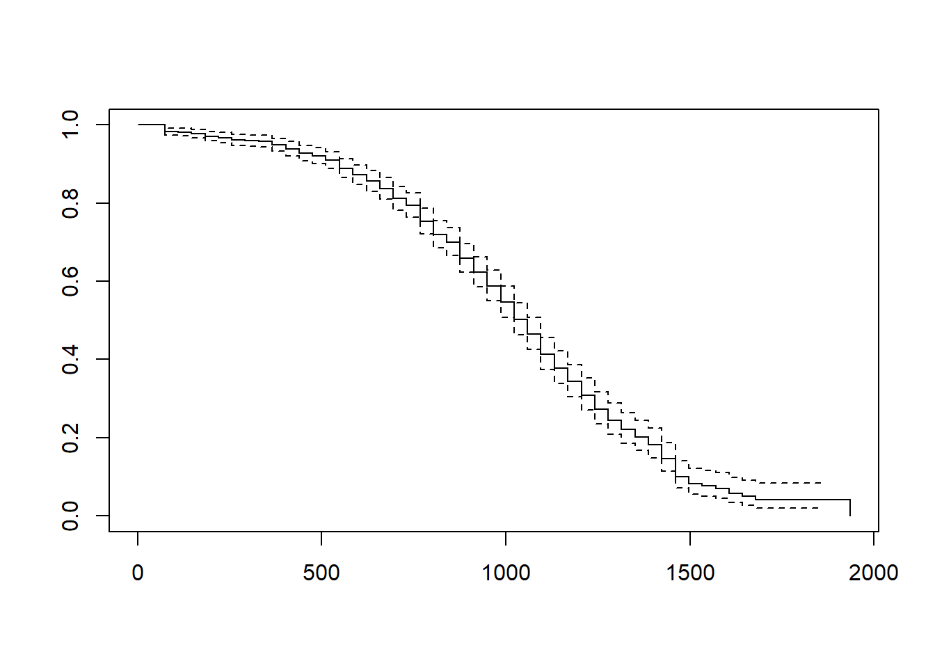
The case associated with row number 6 has the highest Cook’s distance value, followed by the cases associated with row numbers 1 and 66. The cases associated with row numbers 6 and 1 seem to be clearest potential outliers of the three.
We can also print the cases with the highest Cook’s distances. Let’s create an object called cooksD that we will assign a vector of Cook’s distance values to using the cooks.distance function from base R. Just enter the name of the logistic regression model object (model1) as the sole parenthetical argument. Next, update the object we called cooksD by applying the sort function from base R and entering the cooksD object as the first object and decreasing=TRUE as the second argument; this will sort the Cook’s distance values in descending order. Finally, apply the head function from base R, and as the first argument enter the name of the cooksD object that we just sorted; as the second argument, type n=20 to show the top 20 rows, as opposed to the default top 6 rows.
# Estimate Cook's distance values
cooksD <- cooks.distance(model2)

# Sort Cook's distance values in descending order
cooksD <- sort(cooksD, decreasing=TRUE)

# View top 20 Cook's distance values
head(cooksD, n=20)
## 6 1 66 42 96 74 27 26 67 61 68 4
## 0.15184792 0.13426790 0.10091817 0.08227834 0.05869871 0.04691783 0.04554332 0.04249992 0.03973226 0.02634920 0.02182251 0.01882168
## 25 52 54 69 8 75 77 64
## 0.01802907 0.01720366 0.01718997 0.01718628 0.01661234 0.01611474 0.01593173 0.01552323Again, we see cases associated with row numbers 6 (.152), 1 (.134), and 66 (.101) having the highest Cook’s distance values. As a sensitivity analysis, we could estimate our model once more after removing the cases associated with row numbers 6 and 1 (and maybe even 66) from our data frame. With that being said, we should be wary of removing outlier or influential cases and should do so only when we have good justification for doing so. A liberal threshold Cook’s distance is 1, which means that we would grow concerned if any of these values exceeded 1, whereas a more conservative threshold is 4 divided by the sample size (4 / 98 = .041). These Cook’s distance values are all well-below the more liberal threshold, so I would say we’re safe to leave the associated cases in the data.
No (Multi)Collinearity Between Predictor Variables: To assess whether (multi)collinearity might be an issue, let’s estimate two indices of collinearity: tolerance and valence inflation factor (VIF). If you haven’t already, install the car package (Fox and Weisberg 2019) which contains the vif function we will use to compute tolerance.
Now, access the car package using the library function.
Apply the vif function to the model object (model2).
##       JS     NAff       TI
## 1.068428 1.020933 1.067496
Next, the tolerance statistic is just the reciprocal of the VIF (1/VIF), and generally, I find it to be easier to interpret because the tolerance statistic represents the shared variance (R2) of just the predictor variables in a single model (excluding the outcome variable) and subtracting that value from 1 (1 - R2), where a focal predictor variable serves as the outcome and the other(s) (collectively) explain variance in that predictor variable. We typically get concerned when the tolerance statistics approach .20, as the closer it gets to .00, the higher the collinearity. Ideally, we want the tolerance statistic to approach 1.00, as this indicates that there are lower levels of collinearity. To compute the tolerance statistic, we just divide 1 by the VIF.
##        JS      NAff        TI
## 0.9359549 0.9794966 0.9367719
This table indicates that there are low levels of collinearity. Specifically, we can see that the tolerance statistics are all closer to 1.00 and definitely above .20, thereby indicating that collinearity is not likely an issue.
Association Between Any Continuous Predictor Variable and Logit Transformation of Outcome Variable Is Linear: To test the assumption of linearity between a continuous predictor variable and the logit transformation of the outcome variable, we can add to the model the interaction term between any continuous predictor variable and its logarithmic (i.e., natural log) transformation. [Note: We do not perform the following test/approach for categorical predictor variables.] We will use an approach that is commonly referred to as the Box-Tidwell approach (Hosmer and Lemeshow 2000). To apply this approach, we need to add the interaction term between each predictor variable and its logarithmic transformation to our logistic regression model – but not the main effect for the logarithmic transformation of the predictor variable. In our regression model formula, specify the dichotomous outcome variable Turnover to the left of the ~ symbol. To the right of the ~ symbol, type the name of each predictor variable JS followed by the + symbol. After the + symbol, type the name of the same predictor variable JS, followed by the : symbol and the log function from base R with the predictor variable as its sole parenthetical argument. Repeat that process for all continuous predictor variables in the model. Be sure to name the model object, and here I name it arbitrarily boxtidwell. Finally, use the summary function from base R to generate the model output, and within the parentheses, enter the name of the model you created in the prior step (boxtidwell).
# Box-Tidwell diagnostic test of linearity between continuous predictor variables and
# logit transformation of outcome variable
boxtidwell <- glm(Turnover ~ JS + JS:log(JS) + NAff + NAff:log(NAff) + TI + TI:log(TI),
                  data=td, family=binomial)

# Print summary of results
summary(boxtidwell)
##
## Call:
## glm(formula = Turnover ~ JS + JS:log(JS) + NAff + NAff:log(NAff) +
## TI + TI:log(TI), family = binomial, data = td)
##
## Coefficients:
## Estimate Std. Error z value Pr(>|z|)
## (Intercept) 0.9206 9.8331 0.094 0.9254
## JS -4.5845 2.6176 -1.751 0.0799 .
## NAff -0.4107 6.4047 -0.064 0.9489
## TI 3.2888 3.0158 1.091 0.2755
## JS:log(JS) 2.0053 1.1844 1.693 0.0904 .
## NAff:log(NAff) 0.9559 3.5321 0.271 0.7867
## TI:log(TI) -1.2101 1.5232 -0.794 0.4269
## ---
## Signif. codes: 0 '***' 0.001 '**' 0.01 '*' 0.05 '.' 0.1 ' ' 1
##
## (Dispersion parameter for binomial family taken to be 1)
##
## Null deviance: 127.02 on 94 degrees of freedom
## Residual deviance: 100.85 on 88 degrees of freedom
## (4 observations deleted due to missingness)
## AIC: 114.85
##
## Number of Fisher Scoring iterations: 5Because the p-values associated with each of the interaction terms and their regression coefficients (JS:log(JS), NAff:log(NAff), TI:log(TI)) are equal to or greater than the conventional two-tailed alpha level of .05, we have no reason to believe that any of the associations between the continuous predictor variables and the logit transformation of the outcome variable are nonlinear. If one of the interaction terms had been statistically significant, then we might have evidence that the assumption was violated, meaning we would assume a nonlinear association instead, and one potential solution would be to apply a transformation to the predictor variable in question (e.g., logarithmic transformation). Finally, we only apply this test when the predictor variables in question are continuous (interval, ratio).
Important Note: If the variable for which you are applying the Box-Tidwell approach described above has one or more cases with a score of zero, then you will receive an error message when you run the model with the log function. The reason for the error is that the log of zero or any negative value is (mathematically) undefined. There are many reasons why your variable might have cases with scores equal to zero, some of which include: (a) zero is a naturally occurring value for the scale on which the variable is based, or (b) the variable was grand-mean centered or standardized, such that the mean is now equal to zero. There are some approaches to dealing with this issue and neither approach I will show you is going to be perfect, but each approach will give you an approximate understanding of whether violation of the linearity assumption might be an issue. First, we can add a positive numeric constant to every score on the continuous predictor variable in question that will result in the new lowest score being 1. Why 1 you might ask? Well, the rationale is somewhat arbitrary; the log of 1 is zero, and there is something nice about grounding the lowest logarithmic value at 0. Due note, however, that the magnitude of the linear transformation will have some effect on the p-value associated with the Box-Tidwell interaction term. Second, if there are proportionally very few cases with scores of zero on the predictor variable in question, we can simply subset those cases out for the analysis. These approaches to addressing zero values (including the error message you might encounter) are demonstrated in a previous section on simple logistic regression.
48.3.4.2 Interpret Model Results
Now we’re ready to interpret the results of the multiple logistic regression model. For clarity, let’s re-specify our original simple logistic regression model from above. To apply the glm function, type the name of the function. As the first argument, specify the logistic regression model, wherein the dichotomous outcome variable is typed to the left of the ~ symbol, and the predictor variables are typed to the right of the ~ symbol, with each predictor variable separated by the + operator. As the second argument, type data= followed by the name of the data frame (td) to which both of the variables belong. Third, type the argument family=binomial, which by default estimates a logit (logistic) model. Be sure to name and create an object based on your model using the <- assignment operator; here, I again arbitrarily named the object model2. Finally, use the summary function from base R to generate the model output, and within the parentheses, enter the name of the model you created in the prior step (model2).
# Estimate multiple logistic regression model
model2 <- glm(Turnover ~ JS + NAff + TI, data=td, family=binomial)

# Print summary of results
summary(model2)
##
## Call:
## glm(formula = Turnover ~ JS + NAff + TI, family = binomial, data = td)
##
## Coefficients:
## Estimate Std. Error z value Pr(>|z|)
## (Intercept) -3.9286 1.8120 -2.168 0.03015 *
## JS -0.2332 0.2215 -1.053 0.29253
## NAff 1.1952 0.4996 2.392 0.01674 *
## TI 0.8967 0.3166 2.832 0.00462 **
## ---
## Signif. codes: 0 '***' 0.001 '**' 0.01 '*' 0.05 '.' 0.1 ' ' 1
##
## (Dispersion parameter for binomial family taken to be 1)
##
## Null deviance: 127.02 on 94 degrees of freedom
## Residual deviance: 105.23 on 91 degrees of freedom
## (4 observations deleted due to missingness)
## AIC: 113.23
##
## Number of Fisher Scoring iterations: 4The output generates the model coefficient estimates and model fit (i.e., AIC) information.
To estimate the 95% confidence intervals for the regression coefficients based on their standard errors, we can apply the confint function from base R with the name of our model as the sole argument (model2).
## Waiting for profiling to be done...## 2.5 % 97.5 %
## (Intercept) -7.6905274 -0.5144811
## JS -0.6793832 0.1980706
## NAff 0.2606377 2.2375600
## TI 0.3091687 1.5633542Coefficients: The Coefficients section of the output from the summary of the glm function generates the model coefficient estimates and model fit (i.e., AIC) information, and the output from the confint provides the confidence intervals. To begin, the Coefficients section displays the regression coefficients (slopes, weights) and their standard errors, z-values, and p-values. Typically, the intercept value and its significance test are not of interest, unless we wish to use the value to specify the regression model equation. The estimate of the unstandardized regression coefficient for the predictor variable (JS) in relation to the logit transformation of the outcome variable (Turnover) is not statistically significant when controlling for the other predictor variables in the model because the associated p-value is equal to or greater than .05 (b = -.233, p = .293, 95% CI[-0.667, .201]). The regression coefficient for NAff is 1.195 and its associated p-value is less than .05, indicating that the association is statistically significant when controlling for the other predictor variables in the model (b = 1.195, p = .017, 95% CI[.216, 2.174]). Finally, the regression coefficient for TI is .897 and its associated p-value is less than .05, indicating that the association is also statistically significant when controlling for the other predictor variables in the model (b = .897, p = .005, 95% CI[.276, 1.517]).
Given that one of the predictor variables did not share a statistically significant association with the outcome when included in the model, we typically would not write out the regression equation with that variable included. Instead, we would typically re-estimate the model without that variable. For illustrative purposes, however, we will write out the equation. Using the intercept and predictor variable coefficient estimates, we can write out the equation for the regression model as follows:
\(\ln(\frac{p}{1-p}) = -3.929 - .233 \times JS_{observed} + 1.195 \times NAff_{observed} + .897 \times TI_{observed}\)
where \(p\) refers to, in this example, as the probability of quitting.
If you recall from earlier in the tutorial, we can also interpret our findings with respect to \(\log(odds)\).
\(\log(odds) = \ln(\frac{p}{1-p}) = -3.929 - .233 \times JS_{observed} + 1.195 \times NAff_{observed} + .897 \times TI_{observed}\)
To that end, to aid our interpretation of the significant finding, we can convert our logistic regression coefficient to an odds ratio by simply exponentiating it – for example:
\(e^{1.195} = 3.304\)
We can also do this using R by applying the exp function from base R. Specifically, within the exp function parentheses, type the name of the coef function from base R, which extracts the regression coefficients from the model object. As the sole argument within the coef function parentheses, enter the name of the model we previously specified (model2).
## (Intercept)          JS        NAff          TI
##   0.0196714   0.7919969   3.3041473   2.4513941
We should only interpret those odds ratios in which their corresponding regression coefficient was statistically significant; accordingly, in this example, we will just interpret the odds ratios belonging to NAff and TI. Regarding NAff, its odds ratio of 3.304 is greater than 1, which implies a positive association between the predictor and the outcome variables, which we already knew from the negative regression coefficient on which it is based. Thus, the odds of quitting are 3.304 times as likely for every one unit increase in NAff when controlling for other predictor variables in the model. Regarding TI, its odds ratio of 2.451 is also greater than 1, and thus, the odds of quitting are 2.451 times as likely for every one unit increase in TI when controlling for other predictor variables in the model. Note that the odds ratio (OR) is a type of effect size, and thus we can compare odds ratios and describe an odds ratio qualitatively using descriptive language. There are different rules of thumb, and for the sake of parsimony, I provide rules of thumb for when odds ratios are greater than 1 and less than 1. Both odds ratios are about medium in terms of their magnitude.
| Odds Ratio > 1 | Odds Ratio < 1 | Description |
|---|---|---|
| 1.2 | .8 | Small |
| 2.5 | .4 | Medium |
| 4.3 | .2 | Large |
To get the 95% confidence intervals for the odds ratio, we can nest the confint function within the exp function.
## Waiting for profiling to be done...## 2.5 % 97.5 %
## (Intercept) 0.000457137 0.5978107
## JS 0.506929579 1.2190484
## NAff 1.297757439 9.3704394
## TI 1.362292195 4.7748100Model Fit & Performance: Returning to the original output of the multiple logistic regression model, let’s examine the section that contains information about model fit. Note that we don’t have an estimate of R-squared (R2) like we would with a traditional linear regression model. Later on, we will compute the pseudo-R-squared (R2) value. As you can see in the output, we get the null deviance and residual deviance values (and their degrees of freedom) as well as the Akaike information criterion (AIC) value. If we add 1 to the degrees of freedom of our null deviance estimate, we get the number of cases retained for the analysis (N = 95). By themselves, these values are not very meaningful; however, they can be used to compare nested models, which is beyond the scope of this tutorial.
For our purposes, we will assess the model’s fit to the data initially by creating a confusion matrix in which we display the model’s accuracy in predicting the outcome. Before doing so, recall that in our analysis above, we lost one case because of missing data on either the predictor, outcome, or both, which dropped our sample size from 99 to 95 for the analysis. Thus, we should drop the cases with missing data prior to estimating our baseline data and confusion matrix. We’ll start by using the subset function from base R to select just the variables from our data frame that we used in our logistic regression model: Turnover, JS, NAff, and TI. As the first argument, type the name of the data frame (td). As the second argument, type select= followed by the c (combine) function from base R. Within the c function parentheses, enter the names of the two variables we wish to retain (Turnover, JS). Using the <- assignment operator, create a new data frame object, and here I arbitrarily call this object td_short.
# Create new short data frame with just the retained variables
td_short <- subset(td, select=c(Turnover, JS, NAff, TI))
Next, apply the na.omit function from base R to drop cases in our data frame that are missing values on one or more variables. In the function parentheses, enter the name of the data frame we just created (td_short). Using the <- assignment operator, overwrite the td_short data frame by entering its name to the left of the <- assignment operator.
There are different ways we can estimate our baseline, but let’s keep it simple and use the xtabs function from base R. As the first argument, type the ~ followed the name of the short data frame td_short, followed by the $ and the outcome variable (Turnover). Use the <- operator to create and name a new table object, where here I arbitrarily call it table1. Use the print function to view the table object (table1). Remember that for the Turnover variable quit = 1 and stay = 0.
# Number of cases at each level of outcome variable
table1 <- xtabs(~ td_short$Turnover)

# Print the table
print(table1)
## td_short$Turnover
## 0 1
## 37 58As you can see, 37 people actually stayed and 58 people actually quit. To convert these to proportions, apply the prop.table function from base R to the table object we created in the previous step (table1).
## td_short$Turnover
##         0         1
## 0.3894737 0.6105263
Based on this output, we see that 38.9% of people stayed and 61.1% quit.
Now we’re ready to estimate the predicted probabilities of someone quitting based on our logistic regression model. Begin by specifying the name of the object to which you want to assign the vector of predicted probabilities (pred.prob), using the <- assignment operator. Next, type the name of the predict function from base R. As the first argument, type the name of our logistic regression model (model2). As the second argument, enter the argument type="response" to indicate that you want to predict the outcome (response) variable.
We now need to dichotomize the vector of predicted probabilities (pred.prob), such that any case with a predicted probability of .50 or higher is assigned a 1 (quit), and any case with a predicted probability that is less than .50 is assigned a 0 (stay). That is, we’re setting our threshold for experiencing the event in question as .50. As the first step, let’s create a new vector called dich.pred.prob (or whatever you would like to call it) based on the values from the pred.prob vector you created in the previous step. Next, for the dich.pred.prob, dichotomize the values as either a 1 or a 0 in accordance with the approach described above. For more information on the data-management operations below, check out chapter on cleaning data.
# Dichotomize probabilities, where .50 or greater is 1 (quit) and less than .50 is 0 (stay)
dich.pred.prob <- pred.prob
dich.pred.prob[dich.pred.prob >= .50] <- 1
dich.pred.prob[dich.pred.prob < .50] <- 0
Building on the xtabs function from above, use the + symbol to add the new dich.pred.prob vector as the column variable in the table. Also, create a new table object using the <- operator called table2 (or whatever you would like to call it). Use the print function to print the table2 object.
# Number of cases at each level of outcome variable
table2 <- xtabs(~ td_short$Turnover + dich.pred.prob)
print(table2)
## dich.pred.prob
## td_short$Turnover 0 1
## 0 23 14
## 1 6 52This table is our confusion matrix, where the rows represent the actual turnover observations (i.e., true state of affairs), and the columns represent the predicted turnover occurrences. In other words, a cross-tabulation is shown in which the rows represent actual/observed turnover behavior (0 = stay, 1 = quit), and the columns represent predicted turnover behavior (0 = stay, 1 = quit). Thus, the cross-tabulation (i.e., confusion matrix) helps us understand how accurate our model predictions were relative to the observed data, thereby providing us with an indication of how well the model fit the data.
By applying the prop.table function, we can calculate the row proportions, which will give us an idea of how accurately our logistic regression model classified people as staying and as leaving relative to the actual, observed data for turnover. As the first argument, type the name of the table object (table2), and as the second argument, enter the numeral 1 to indicate that we want the row proportions.
##                  dich.pred.prob
## td_short$Turnover         0         1
##                 0 0.6216216 0.3783784
##                 1 0.1034483 0.8965517
Of those who actually stayed (0), we were able to predict their turnover behavior with 62.2% accuracy using our model. Of those who actually quit (1), our model even better, as we were able to predict that outcome with 89.7% accuracy. Not too shabby.
Finally, let’s determine the percentage of correct classifications (i.e., model accuracy) for both quit and stay behavior. In other words, we want to determine the percentage of correct decisions that were made based on our model relative to the overall number of decisions made by our model (i.e., sample size). We will use basic arithmetic to do so. First, specify the numerator value, which will be calculated by adding those correct predictions; in this context, the correct decisions are those in which the model accurately predicted who would stay (0) and who would quit (1). Thus, we’re interested in the cells that correspond to 0 on the Turnover variable and 0 on the dich.pred.prob vector, which is the upper-left cell in our 2x2 table. To reference that cell and its value, type the name of the table object (table2), and within brackets beside it ([ ]), type the name of the row label (“0”), followed by a comma and the name of the column label (“0”). To reference the lower-right cell, which represents the number of correct predictions regarding quitting, type the name of the table object (table2), and within brackets beside it ([ ]), type the name of the row label (“1”), followed by a comma and the name of the column label (“1”). Now add those together to form the numerator. In the denominator, apply the sum function from base R to the table object (table2) to calculate how many predictions were made - or in other words, the sample size for those who had data for both the predictor variable (JS) and the outcome variable (Turnover) in our original model.
# Estimate overall percentage of correct classifications
(table2["0","0"] + table2["1","1"]) / sum(table2)
## [1] 0.7894737The overall percentage of correct classifications 78.9%, which is a pretty good accuracy in prediction when using the three predictor variables in our model. If we were to add additional predictor variables to the model, our hope would be that our percentage of correct predictions would increase to a notable extent.
Nagelkerke pseudo-R2: To compute Nagelkerke’s pseudo-R2, we will need to install and access the DescTools package so that we can use its PseudoR2 function.
In the PseudoR2 function, we will specify the name of the model object (model2) as the first argument. As the second argument, type "Nagel" to request pseudo-R2 calculated using Nagelkerke’s formula.
## Nagelkerke
##  0.2779516
The estimated Nagelkerke pseudo-R2 is .278, which is a big improvement over the simple logistic regression model we estimated above for which pseudo-R2 was just .073. Remember, a pseudo-R2 is not the exact same thing as a true R2, so we should interpret it with caution. With caution, we can conclude that JS, NAff, and TI explain 27.8% of the variance in Turnover.
Because the DescTools package also has a function called Logit, let’s detach the package before moving forward so that we don’t inadvertently attempt to use the Logit function from DescTools as opposed to the one from lessR.
Technical Write-Up of Results: A turnover study was conducted based on a sample of 99 employees from the past year, some of whom quit the company and some of whom stayed. Turnover behavior (quit vs. stay) (Turnover) is our outcome of interest, and because it is dichotomous, we used logistic regression. We, specifically, were interested in the extent to which employees’ self-reported job satisfaction, negative affectivity, and turnover intentions were associated with their decisions to quit or stay, and thus all three were was used as continuous predictor variables in our multiple logistic regression model. In total, due to missing data, 95 employees were included in our analysis. Results indicated that, indeed, job satisfaction was not associated with turnover behavior to a statistically significant extent (b = -.233, p = .293, 95% CI[-0.667, .201]). Negative affectivity, however, was positively and significantly associated with turnover behavior (b = 1.195, p = .017, 95% CI[.216, 2.174]), such that the odds of quitting were 3.304 times as likely for every one unit increase in negative affectivity, when controlling for other predictor variables in the model. Similarly, turnover intentions were also positively and significantly associated with turnover behavior (b = .897, p = .005, 95% CI[.276, 1.517]), such that the odds of quitting were 2.451 times as likely for every one unit increase in turnover intentions, when controlling for other predictor variables in the model. Both of these significant associations were medium in magnitude. Overall, based on our estimated multiple logistic regression model, we were able to predict actual turnover behavior in our sample with 78.9% accuracy. Finally, the estimated Nagelkerke pseudo-R2 was .278. We can cautiously conclude that job satisfaction, negative affectivity, and turnover intentions explain 27.8% of the variance in voluntary turnover.
Standardizing Continuous Predictor Variables: Optionally, sometimes we may decide to standardize the continuous predictor variables in our model, as this may make it easier to compare the odds ratios between variables. To do so, we just need to apply the scale function to the continuous predictor variable in the model. For more information on standardizing variables, please check out the chapter on centering and standardizing variables.
# Estimate simple logistic regression model
# with standardized continuous predictor variable
model2_b <- glm(Turnover ~ scale(JS) + scale(NAff) + scale(TI),
                data=td, family=binomial)

# Print summary of results
summary(model2_b)
##
## Call:
## glm(formula = Turnover ~ scale(JS) + scale(NAff) + scale(TI),
## family = binomial, data = td)
##
## Coefficients:
## Estimate Std. Error z value Pr(>|z|)
## (Intercept) 0.5669 0.2415 2.348 0.01888 *
## scale(JS) -0.2675 0.2542 -1.053 0.29253
## scale(NAff) 0.6190 0.2588 2.392 0.01674 *
## scale(TI) 0.7685 0.2713 2.832 0.00462 **
## ---
## Signif. codes: 0 '***' 0.001 '**' 0.01 '*' 0.05 '.' 0.1 ' ' 1
##
## (Dispersion parameter for binomial family taken to be 1)
##
## Null deviance: 127.02 on 94 degrees of freedom
## Residual deviance: 105.23 on 91 degrees of freedom
## (4 observations deleted due to missingness)
## AIC: 113.23
##
## Number of Fisher Scoring iterations: 448.3.4.3 Compute Predicted Probabilities
When creating a confusion matrix above, we already estimated the predicted probabilities of the model when applied to the sample on which it was estimated; however, we didn’t append this new vector to of values to our data frame object (td). For the sake of clarity, we will re-do this step using the predict function from base R once more. We’ll begin by specifying the name of the object to which you want to assign the vector of predicted probabilities (pred.prob), using the <- assignment operator. Next, type the name of the predict function from base R. As the first argument, type the name of our logistic regression model (model1). As the second argument, enter the argument type="response" to indicate that you want to predict the outcome (response) variable.
# Estimate predicted probabilities based on
# sample used to estimate the logistic regression model
pred.prob <- predict(model2, type="response")
Now let’s add the pred.prob vector as a new variable called pred.prod.allpred in the td data frame object.
- Let’s overwrite the existing
tddata frame object by using the<-assignment operator. - Specify the name of the
mergefunction from base R. For more information on this function, please refer to this chapter supplement from the chapter on joining data frames.
- As the first argument in the
mergefunction, specifyx=followed by the name of thetddata frame object. - As the second argument in the
mergefunction, specifyy=followed by thedata.framefunction from base R. As the sole argument within thedata.framefunction specify a name for the new variable that will contain the predicted probabilities based onJSscores (pred.prod.allpred), followed by the=operator and the name of the vector object containing the predicted probabilities (pred.prod). - As the third argument in the
mergefunction, typeby="row.names", which will match rows from thexandydata frame objects based on their respective row names (i.e., row numbers). - As the fourth argument in the
mergefunction, typeall=TRUEto request a full merge, such that all rows with data will be retained from both data frame objects when merging.
# Simple logistic regression model with predicted probabilities
# added as new variable in existing data frame object
td <- merge(x=td,
            y=data.frame(
              pred.prod.allpred = pred.prob),
            by="row.names",
            all=TRUE)
If we print the first six rows from the td data frame object, we will see the new column containing the predicted probabilities based on our simple logistic regression model.
##   Row.names Row.names     ID Turnover   JS   OC   TI NAff JS_0 JS_1 pred.prob.JS dich.pred.prob.JS pred.prod.allpred
## 1         1         1 EMP559        1 4.96 5.32 0.51 1.87 4.73 5.73    0.4216566                 0        0.08371016
## 2        10        18 EMP643        1 3.35 2.94 3.60 2.08 3.12 4.12    0.5960009                 1        0.73187048
## 3        11        19 EMP644        1 2.33 0.80 3.22 2.45 2.10 3.10    0.6974856                 1        0.79306191
## 4        12         2 EMP561        1 1.72 1.47 4.08 2.48 1.49 2.49    0.7507079                 1        0.90827169
## 5        13        20 EMP647        0 2.98 2.16 2.41 2.32 2.75 3.75    0.6343220                 1        0.57694329
## 6        14        21 EMP677        0 4.64 2.92 1.48 2.43 4.41 5.41    0.4561403                 0        0.31447250
We can now dichotomize the predicted probabilities (pred.prod.allpred), such that any case with a predicted probability of .50 or higher is assigned a 1 (quit), and any case with a predicted probability that is less than .50 is assigned a 0 (stay). That is, we’re setting our threshold for experiencing the event in question as .50. As the first step, let’s create a new variable called dich.pred.prod.allpred (or whatever we would like to call it) based on the values from the pred.prod.allpred variable we just created. Next, for the dich.pred.prod.allpred, dichotomize the values as either a 1 or a 0 in accordance with the approach described above. For more information on the data-management operations below, check out chapter on cleaning data.
# Dichotomize probabilities, where .50 or greater is 1 (quit) and less than .50 is 0 (stay)
td$dich.pred.prod.allpred <- td$pred.prod.allpred
td$dich.pred.prod.allpred[td$dich.pred.prod.allpred >= .50] <- 1
td$dich.pred.prod.allpred[td$dich.pred.prod.allpred < .50] <- 0## Row.names Row.names ID Turnover JS OC TI NAff JS_0 JS_1 pred.prob.JS dich.pred.prob.JS pred.prod.allpred
## 1 1 1 EMP559 1 4.96 5.32 0.51 1.87 4.73 5.73 0.4216566 0 0.08371016
## 2 10 18 EMP643 1 3.35 2.94 3.60 2.08 3.12 4.12 0.5960009 1 0.73187048
## 3 11 19 EMP644 1 2.33 0.80 3.22 2.45 2.10 3.10 0.6974856 1 0.79306191
## 4 12 2 EMP561 1 1.72 1.47 4.08 2.48 1.49 2.49 0.7507079 1 0.90827169
## 5 13 20 EMP647 0 2.98 2.16 2.41 2.32 2.75 3.75 0.6343220 1 0.57694329
## 6 14 21 EMP677 0 4.64 2.92 1.48 2.43 4.41 5.41 0.4561403 0 0.31447250
## dich.pred.prod.allpred
## 1 0
## 2 1
## 3 1
## 4 1
## 5 1
## 6 0It’s important to keep in mind that these predicted probabilities are estimated based on the same data we used to estimate the model in the first place. Given this, I would describe this process as predict-ish analytics as opposed to true predictive analytics. To reach predictive analytics, we would need to obtain “fresh” data on the predictor variables, which we could then use to plug into our model; to do this with a model estimated using the glm model, will create a toy data frame with “fresh” predictor variable values sampled from the same population. In a real life situation, we would more than likely read in a new data file and assign that to an object – just like we did in the chapter on applying a compensatory approach to selection decisions using multiple linear regression.
In this toy data frame that we’re naming fresh_td, we use the data.frame function from base R. As the first argument, we’ll create an ID variable with some fictional employee ID numbers. As the second argument, we’ll create a JS variable with some fictional job satisfaction scores. As the third argument, we’ll create a NAff variable with some fictional negative affectivity scores. As the fourth argument, we’ll create a TI variable with some fictional turnover intentions scores.
# Create toy data frame object for illustration purposes
fresh_td <- data.frame(ID=c("EMP1000","EMP1001","EMP1002",
                            "EMP1003","EMP1004","EMP1005"),
                       JS=c(4.5, 1.6, 0.7,
                            5.9, 2.1, 3.0),
                       NAff=c(0.9, 3.3, 6.0,
                            4.2, 4.0, 1.9),
                       TI=c(6.0, 5.5, 4.8,
                            3.0, 0.1, 1.1))
When estimating the predicted probabilities of turnover based on these new predictor variable scores, we’ll do the following:
- Using the
<-assignment operator, we will create a new variable calledprob_allpredthat we will append to thefresh_tdtoy data frame object (using the$operator). - To the right of the
<-assignment operator, type the name of thepredictfunction from base R.
- As the first argument, type the name of the logistic regression model object we estimated using the
td(original) data frame. - As the second argument, type
newdata=followed by the name of the data frame object containing “fresh” data (fresh_td). It’s important that the predictor variable name is the same in this data frame as it is in the original data frame on which the model was estimated. - As the third argument, insert
type="response", which will request the predicted probabilities.
# Use multiple logistic regression model to estimate
# predicted probabilities of turnover for "fresh" data
fresh_td$prob_allpred <- predict(model2, # name of logistic regression model
                                 newdata=fresh_td, # name of "fresh" data frame
type="response")## ID JS NAff TI prob_allpred
## 1 EMP1000 4.5 0.9 6.0 0.8142131
## 2 EMP1001 1.6 3.3 5.5 0.9897887
## 3 EMP1002 0.7 6.0 4.8 0.9993788
## 4 EMP1003 5.9 4.2 3.0 0.9172278
## 5 EMP1004 2.1 4.0 0.1 0.6111323
## 6 EMP1005 3.0 1.9 1.1 0.2024548