Chapter 57 Evaluating Measurement Models Using Confirmatory Factor Analysis

In this chapter, we will learn how to evaluate measurement models using confirmatory factor analysis (CFA), where CFA is part of the structural equation modeling (SEM) family of analyses. Specifically, we will learn how to evaluate the measurement structure and construct validity of a theoretical construct operationalized as a multi-item measure (i.e., scale, inventory, test, questionnaire).

57.1 Conceptual Overview

Link to conceptual video: https://youtu.be/lhyDp2HtDiA

Confirmatory factor analysis (CFA) is a latent variable modeling approach and is part of the structural equation modeling (SEM) family of analyses, which are also referred to as covariance structure analyses. CFA is a useful statistical tool for evaluating the internal structure of a measure designed to assess a theoretical construct (i.e., concept); in other words, we can apply CFA to evaluate the construct validity of a construct. CFA allows us to directly specify and estimate a measurement model, which ultimately can be incorporated into structural regression models.

In CFA models, constructs are represented as latent variables (i.e., latent factors), which by nature are not directly measured. Instead, observed (manifest) variables serve as indicators of the latent construct. I should note that in this chapter, we will focus exclusively on reflective measurement models, which are models in which the latent factor is specified as the direct cause of its indicators. Not covered in this chapter are formative measurement models, which are models in which the observed variables are specified as the direct causes of the latent factor.

57.1.1 Path Diagrams

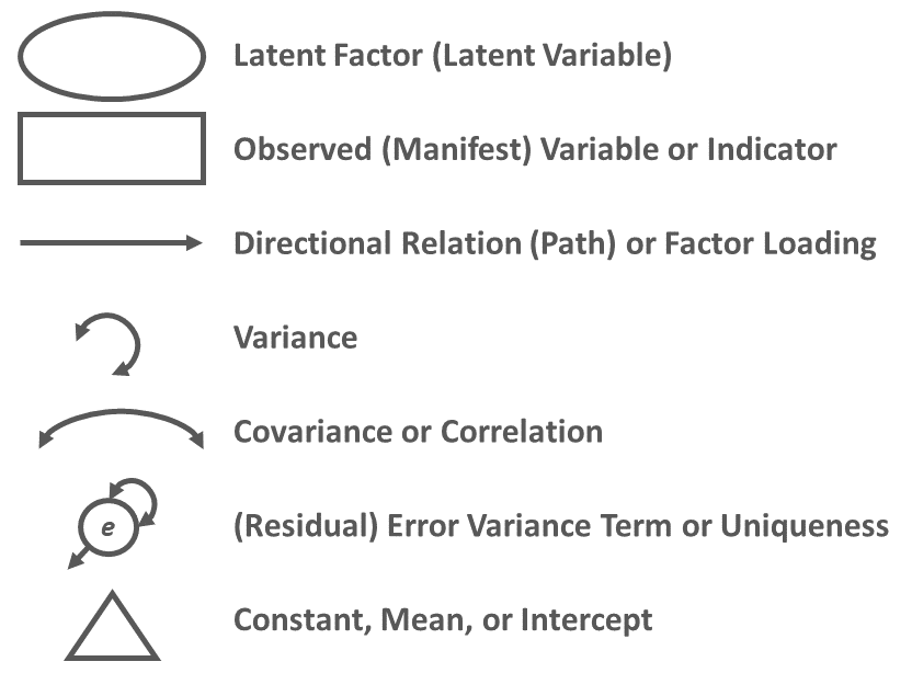
It is often helpful to visualize a CFA model using a path diagram. A path diagram displays the model parameter specifications and can also include parameter estimates. Conventional path diagram symbols are shown in Figure 1.

Figure 1: Conventional path diagram symbols and their meanings.

For an example of how the path diagram symbols can be used to construct a visual depiction of a CFA model, please reference Figure 2. The path diagram depicts a one-factor CFA model for a multi-item role clarity measure, which means that the model has a single latent factor representing the psychological construct called role clarity. Further, four observed variables (i.e., Items 1-4) serve as indicators of the latent factor, such that the indicators are reflective of the latent factor. Putting it all together, the one-factor CFA model serves as a measurement model and represents the measurement structure of a four-item measure designed to assess the construct of role clarity.

Figure 2: Example of a one-factor confirmatory factor analysis (CFA) model path diagram.

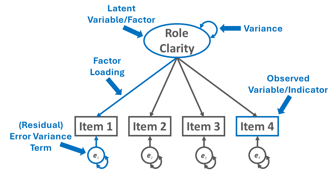
By convention, the latent factor for role clarity is represented by an oval or circle. Please note that the latent factor is not directly measured; rather, we infer information about the latent factor from its four indicators, which in this example correspond to Items 1-4. The latent factor has a variance term associated with it, which represents the latent factor’s variability; in CFA models, we often to don’t spend much time interpreting latent factors’ variance terms, though.

Each of the four observed variables (indicators) is represented with a rectangle. The one-directional, single-sided arrows represent the factor loadings, and point from the latent factor to the observed variables (indicators). Each indicator has a (residual) error variance term, which represents the amount of variance left unexplained by the latent factor in relation to each indicator.

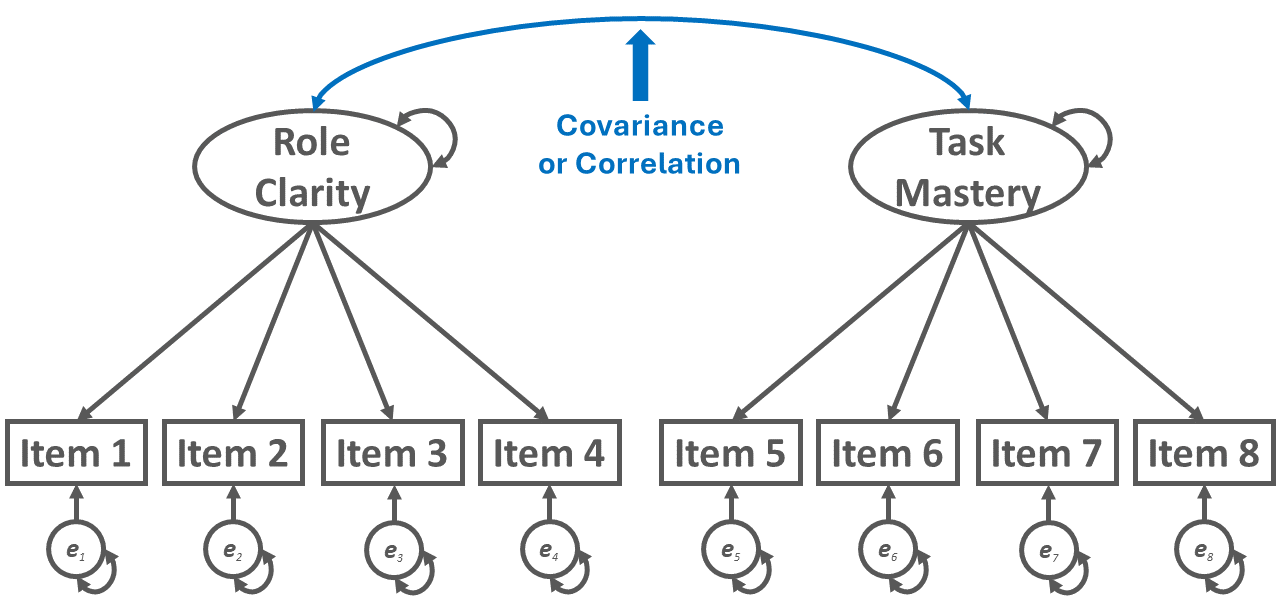
To illustrate the covariance path diagram symbol, let’s refer to Figure 3. When standardized, a covariance can be interpreted as a correlation. The covariance symbol is a double-sided arrow in which the arrows connect two distinct latent or observed variables. In Figure 3, the path diagram depicts a multi-factor CFA model and, more specifically, a two-factor CFA model. The first latent factor is associated with a four-item role clarity measure, and the second latent factor is associated with a four-item task mastery measure. If freely estimated, the covariance term allows the two latent factors to covary with each other.

Figure 3: Example of a multi-factor confirmatory factor analysis (CFA) model path diagram.

57.1.2 Model Identification

Model identification has to do with the number of (free or freely estimated) parameters specified in the model relative to the number of unique (non-redundant) sources of information available, and model implication has important implications for assessing model fit and estimating parameter estimates.

Just-identified: In a just-identified model (i.e., saturated model), the number of freely estimated parameters (e.g., factor loadings, covariances, variances) is equal to the number of unique (non-redundant) sources of information, which means that the degrees of freedom (df) is equal to zero. In just-identified models, the model parameter standard errors can be estimated, but the model fit cannot be assessed in a meaningful way using traditional model fit indices.

Over-identified: In an over-identified model, the number of freely estimated parameters is less than the number of unique (non-redundant) sources of information, which means that the degrees of freedom (df) is greater than zero. In over-identified models, traditional model fit indices and parameter standard errors can be estimated.

Under-identified: In an under-identified model, the number of freely estimated parameters is greater than the number of unique (non-redundant) sources of information, which means that the degrees of freedom (df) is less than zero. In under-identified models, the model parameter standard errors and model fit cannot be estimated. Some might say under-identified models are overparameterized because they have more parameters to be estimated than unique sources of information.

Most (if not all) statistical software packages that allow structural equation modeling (and by extension, confirmatory factor analysis) automatically compute the degrees of freedom for a model or, if the model is under-identified, provide an error message. As such, we don’t need to count the number of sources of unique (non-redundant) sources of information and free parameters by hand. With that said, to understand model identification and its various forms at a deeper level, it is often helpful to practice calculating the degrees freedom by hand when first learning.

The formula for calculating the number of unique (non-redundant) sources of information available for a particular model is as follows:

\(i = \frac{p(p+1)}{2}\)

where \(p\) is the number of observed variables to be modeled. This formula calculates the number of possible unique covariances and variances for the variables specified in the model – or in other words, it calculates the lower diagonal of a covariance matrix, including the variances.

In the single-factor CFA model path diagram specified above, there are four observed variables: Item 1, Item 2, Item 3, and Item 4. Accordingly, in the following formula, \(p\) is equal to 4, and the number of unique (non-redundant) sources of information is 10.

\(i = \frac{4(4+1)}{2} = \frac{20}{2} = 10\)

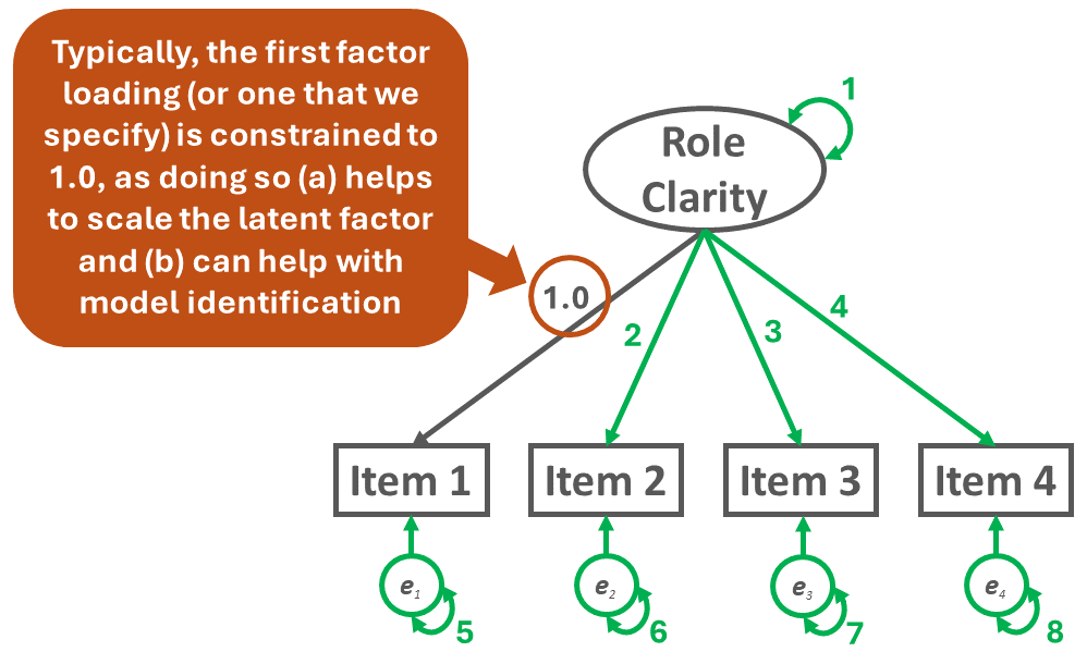
To count the number of free parameters (\(k\)), simply add up the number of the specified unconstrained factor loadings, variances, covariances, and (residual) error variance terms in the one-factor CFA model. Please note that for latent variable scaling and model identification purposes, we typically constrain one of the factor loadings to 1.0, which means that it is not freely estimated and thus doesn’t count as one of the free parameters. As shown in Figure 4 below, the example one-factor CFA model has 8 free parameters.

\(k = 8\)

To calculate the degrees of freedom (df) for the model, we need to subtract the number of free parameters from the number unique (non-redundant) sources of information, which in this example equates to 10 minus 8. Thus, the degrees of freedom for the model is 2, which means the model is over-identified.

\(df = i - k = 10 - 8 = 2\)

Figure 4: Counting the number of free parameters in the CFA model path diagram.

57.1.3 Model Fit

When a model is over-identified (df > 0), the extent to which the specified model fits the data can be assessed using a variety of model fit indices, such as the chi-square (\(\chi^{2}\)) test, comparative fit index (CFI), Tucker-Lewis index (TLI), root mean square error of approximation (RMSEA), and standardized root mean square residual (SRMR). For a commonly cited reference on cutoffs for fit indices, please refer to Hu and Bentler (1999). And for a concise description of common guidelines regarding interpreting model fit indices, including differences between stringent and relaxed interpretations of common fit indices, I recommend checking out Nye (2023). Regardless of which cutoffs we apply when interpreting fit indices, we must remember that such cutoffs are merely guidelines, and it’s possible to estimate an adequate model that meets some but not all of the cutoffs given the limitations of some fit indices. Further, in light of the limitations of conventional model fit index cutoffs, McNeish and Wolf (2023) developed model- and data-specific dynamic fit index cutoffs, which we will cover later in the chapter tutorial.

Chi-square test. The chi-square (\(\chi^{2}\)) test can be used to assess whether the model fits the data adequately, where a statistically significant \(\chi^{2}\) value (e.g., p \(<\) .05) indicates that the model does not fit the data well and a nonsignificant chi-square value (e.g., p \(\ge\) .05) indicates that the model fits the data reasonably well (Bagozzi and Yi 1988). The null hypothesis for the \(\chi^{2}\) test is that the model fits the data perfectly, and thus failing to reject the null model provides some confidence that the model fits the data reasonably close to perfectly. Of note, the \(\chi^{2}\) test is sensitive to sample size and non-normal variable distributions.

Comparative fit index (CFI). As the name implies, the comparative fit index (CFI) is a type of comparative (or incremental) fit index, which means that CFI compares the focal model to a baseline model, which is commonly referred to as the null or independence model. CFI is generally less sensitive to sample size than the chi-square test. A CFI value greater than or equal to .95 generally indicates good model fit to the data, although some might relax that cutoff to .90.

Tucker-Lewis index (TLI). Like CFI, Tucker-Lewis index (TLI) is another type of comparative (or incremental) fit index. TLI is generally less sensitive to sample size than the chi-square test and tends to work well with smaller sample sizes; however, as Hu and Bentler (1999) noted, TLI may be not be the best choice for smaller sample sizes (e.g., N \(<\) 250). A TLI value greater than or equal to .95 generally indicates good model fit to the data, although some might relax that cutoff to .90.

Root mean square error of approximation (RMSEA). The root mean square error of approximation (RMSEA) is an absolute fit index that penalizes model complexity (e.g., models with a larger number of estimated parameters) and thus ends up effectively rewarding more parsimonious models. RMSEA values tend to upwardly biased when the model degrees of freedom are fewer (i.e., when the model is closer to being just-identified); further, Hu and Bentler (1999) noted that RMSEA may not be the best choice for smaller sample sizes (e.g., N \(<\) 250). In general, an RMSEA value that is less than or equal to .06 indicates good model fit to the data, although some relax that cutoff to .08 or even .10.

Standardized root mean square residual (SRMR). Like the RMSEA, the standardized root mean square residual (SRMR) is an example of an absolute fit index. An SRMR value that is less than or equal to .06 generally indicates good fit to the data, although some relax that cutoff to .08.

Summary of model fit indices. The conventional cutoffs for the aforementioned model fit indices – like any rule of thumb – should be applied with caution and with good judgment and intention. Further, these indices don’t always agree with one another, which means that we often look across multiple fit indices and come up with our best judgment of whether the model adequately fits the data. Generally, it is not advisable to interpret model parameter estimates unless the model fits the data reasonably adequately, as a poorly fitting model may be due to model misspecification, an inappropriate model estimator, or other factors that need to be addressed. With that being said, we should also be careful to not toss out a model entirely if one or more of the model fit indices suggest less than acceptable levels of fit to the data. The table below contains the conventional stringent and more relaxed cutoffs for the model fit indices.

Fit Index	Stringent Cutoffs for Acceptable Fit	Relaxed Cutoffs for Acceptable Fit
\(\chi^{2}\)	\(p \ge .05\)	\(p \ge .01\)
CFI	\(\ge .95\)	\(\ge .90\)
TLI	\(\ge .95\)	\(\ge .90\)
RMSEA	\(\le .06\)	\(\le .08\)
SRMR	\(\le .06\)	\(\le .08\)

57.1.4 Parameter Estimates

In CFA models, there are various types of parameter estimates, which correspond to the path diagram symbols covered earlier (e.g., covariance, variance, factor loading). When a model is just-identified or over-identified, we can estimate the standard errors for freely estimated parameters, which allows us to evaluate statistical significance. With most software applications, we can request standardized parameter estimates, which facilitate interpretation.

Factor loadings. When we standardize factor loadings, we obtain estimates for each directional relation between the latent factor and an indicator, including for the factor loading that we likely constrained to 1.0 for latent factor scaling and model identification purposes (see above). When standardized, factor loadings can be interpreted like correlations, and generally we want to see standardized estimate values between .50 and .95 (Bagozzi and Yi 1988). If a standardized factor loading falls outside of that range, we typically investigate whether there is a theoretical or empirical reason for the out-of-range estimate, and we may consider removing the associated indicator if warranted.

(Residual) error variance terms. The (residual) error variance terms, which are also known as disturbance terms or uniquenesses, indicate how much variance is left unexplained by the latent factor in relation to the indicators. When standardized, error variance terms represent the proportion (percentage) of variance that remains unexplained by the latent factor. Ideally, we want to see standardized error variance terms that are less than or equal to .50.

Variances. The variance estimate of the latent factor is generally not a focus when evaluating parameter estimates in a CFA model, as the variance of a latent factor depends on the factor loadings and scaling.

Covariances. In a CFA model, covariances between latent factors help us understand the extent to which they are related (or unrelated). When standardized, a covariance can be interpreted as a correlation.

Average variance extracted (AVE). Although not a parameter estimate, per se, average variance extracted (AVE) is a useful statistic for understanding the extent to which indicator variations can be attributed to the latent factor (Fornell and Larcker 1981). The formula for AVE takes into account the factor loadings and (residual) error variance terms associated with a latent factor. In general, we consider AVE values that are greater than or equal to .50 to be acceptable.

Composite reliability (CR). Like AVE, composite reliability (CR) is not a parameter estimate; instead, it is another useful statistic that helps us understand our CFA model. CR is also known as coefficient omega (\(\omega\)), and it provides an estimate of internal consistency reliability. In general, we consider CR values that are greater than or equal to .70 to be acceptable; however, if the estimate falls between .60 and .70, we might refer to the reliability as questionable but not necessarily unacceptable.

57.1.5 Model Comparisons

When evaluating CFA models, especially multi-factor models, we often wish to evaluate whether a focal model performs better (or worse) than an alternative model. Comparing models can help us arrive at a more parsimonious model that still fits the data well, as well as evaluate the potential multidimensionality of a construct.

As an example, imagine we have a focal model with two latent factors, and unique sets of indicators load onto their respective latent factors. Now imagine that we specify an alternative model that has one latent factor, and all the indicators from our focal model load onto that single latent factor. We can compare those two models to determine whether the alternative model fits the data about the same as our focal model or worse.

When two models are nested, we can perform nested model comparisons. As a reminder, a nested model has all the same parameter estimates of a full model but has additional parameter constraints in place. If two models are nested, we can compare them using model fit indices like CFI, TLI, RMSEA, and SRMR. We can also use the chi-square difference (\(\Delta \chi^{2}\)) test (likelihood ratio test) to compare nested models, which provides a statistical test for nested-model comparisons.

When two models are not nested, we can use other model fit indices like Akaike Information Criterion (AIC) and Bayesian Information Criterion (BIC). With respect to these indices, the best fitting model will have lower AIC and BIC values.

57.1.6 Statistical Assumptions

The statistical assumptions that should be met prior to estimating and/or interpreting a CFA model will depend on the type of estimation method. Common estimation methods for CFA models include (but are not limited to) maximum likelihood (ML), maximum likelihood with robust standard errors (MLM or MLR), weighted least squares (WLS), and diagonally weighted least squares (DWLS). WLS and DWLS estimation methods are used when there are observed variables with nominal or ordinal (categorical) measurement scales. In this chapter, we will focus on ML estimation, which is a common method when observed variables have interval or ratio (continuous) measurement scales. As Kline (2011) notes, ML estimation carries with it the following assumptions: “The statistical assumptions of ML estimation include independence of the scores, multivariate normality of the endogenous variables, and independence of the exogenous variables and error terms” (p. 159). When multivariate non-normality is a concern, the MLM or MLR estimator is a better choice than ML estimator, where the MLR estimator allows for missing data and the MLM estimator does not.

57.1.6.1 Sample Write-Up

As part of a new-employee onboarding survey administered 1-month after employees’ respective start dates, we assessed new employees on three multi-item measures targeting feelings of acceptance, role clarity, and task mastery. Using confirmatory factor analysis (CFA), we evaluated the measurement structure of the three multi-item measures, where each item served as an indicator for its respective latent factor; we did not allow indicator error variances to covary (i.e., the associations were constrained to zero) and, by default, the first indicator for each latent factor was constrained to 1 for estimation purposes and the latent-factor covariances were estimated freely. The three-factor model was estimated using the maximum likelihood (ML) estimator and a sample size of 654 new employees. Missing data were not a concern. We evaluated the model’s fit to the data using the chi-square (\(\chi^{2}\)) test, CFI, TLI, RMSEA, and SRMR model fit indices. The \(\chi^{2}\) test indicated that the model fit the data worse than a perfectly fitting model (\(\chi^{2}\) = 295.932, df = 51, p < .001). Further, the CFI and TLI estimates were .925 and .902, respectively, which did not exceed the more stringent threshold of .95 but did exceed the more relaxed threshold of .90, thereby indicating that model showed marginal fit to the data. Similarly, the RMSEA estimate was .086, which was not below the more stringent threshold of .06 but was below the more relaxed threshold of .10, thereby indicating that model showed marginal fit to the data. The SRMR estimate was .094, which was below both the stringent threshold of .06 and the relaxed threshold of .08, thereby indicating unacceptable model fit to the data. Collectively, the model fit information indicated that model showed mostly marginal fit to the data, which indicated the model may have been misspecified. Excluding the third feelings of acceptance item, the standardized factor loadings ranged from .706 to .846, which means that those item’s standardize factor loadings fell well within the acceptable range of .50-.95; however, the standardized factor loading for the third feelings of acceptance item was .186, which was a great deal outside the acceptable range. Regarding the standardized covariance estimates, the correlation between feelings of acceptance and role clarity latent factors was .248, statistically significant (p < .001), and small-to-medium in terms of practical significance; the correlation between feelings of acceptance and task mastery latent factors was .263, statistically significant (p < .001), and small-to-medium in terms of practical significance; and the correlation between role clarity and task mastery latent factors was .180, statistically significant (p < .001), and small in terms of practical significance. The standardized error variances ranged from .284 to .966, which can be interpreted as proportions of the variance not explained by the latent factor. With the exceptions of the third feelings of acceptance item’s error variance (.966) and the fourth feelings of acceptance item’s error variance (.502), the indicator error variances were less than the recommended .50 threshold, which means that unmodeled constructs did not likely have a notable impact on the vast majority of the indicators. The standardized error variance associated with the third feelings of acceptance item was well above the .50 threshold and its value indicates that the AC latent factor fails to explain 96.6% of the variance in that item, which is unacceptable. Given the third feelings of acceptance item’s unacceptably low standardized factor loading and unacceptably high standardized error variance, we reviewed the item’s content (“My colleagues and I feel confident in our ability to complete work.”) and the feelings of acceptance construct’s conceptual definition (“the extent to which an individual feels welcomed and socially accepted at work”). Because the item’s content does not align with the conceptual definition and because of the unacceptable standardized factor loading and error variance, we decided to drop the third feelings of acceptance prior to re-estimating the model. In contrast, the standardized error variance for the fourth feelings of acceptance item was just above the .50 recommended cutoff, and after reviewing the item’s content (“My colleagues listen thoughtfully to my ideas.”) and the construct’s aforementioned conceptual definition, we determined that the item fits within the conceptual definition boundaries; thus, we decided to retain the fourth feelings of acceptance item. The average variance extracted (AVE) estimates for feelings of acceptance, role clarity, and task mastery were .440, .683, and .578, respectively. The AVE estimates associated with the the role clarity and task mastery latent factors exceeded the conventional threshold (\(\ge\) .50), and thus, we can conclude that those factors showed acceptable levels of AVE. In contrast, the AVE estimate associated with the feelings of acceptance latent factor fell below the .50 cutoff; this unacceptable AVE estimate may be the result of the problematic parameter estimates associated with the third feelings of acceptance item that we noted above. The composite reliability (CR) estimates for feelings of acceptance, role clarity, and task mastery were .788, .866, and .845, respectively, which exceeded the conventional threshold of .70 and thus were deemed acceptable. In sum, the three-factor measurement model showed marginal fit to the data, and CR estimates were acceptable; however, when evaluating the parameter estimates, the standardized factor loading and standardized error variance for the third feelings of acceptance item were both unacceptable; further, while the AVE estimates associated with the role clarity and task mastery latent factors were acceptable, the AVE associated with the feelings of acceptance latent factor was unacceptable, which may be attributable to the low standardized factor loading associated with the third feelings of acceptance.

Subsequently, we re-specified and re-estimated the CFA model by removing the third feelings of acceptance item. In doing so, we found the following. The updated model showed acceptable fit to the data according to CFI (.976), TLI (.968), RMSEA (.052), and SRMR (.032). The chi-square test (\(\chi^{2}\) = 113.309, df = 41, p < .001), however, indicated that the model did not fit the data well; that said, the chi-square test is sensitive to sample size. We concluded that in general the model showed acceptable fit to the data. Standardized factor loadings ranged from .708 to .846, which all fell well within the recommended .50-.95 acceptability range. The standardized error variances for items ranged from .284 to .499, and thus all fell below the target threshold of .50, thereby indicating that it was unlikely that an unmodeled construct had an outsized influence on any of those items. The average variance extracted (AVE) for feelings of acceptance, role clarity, and task mastery were .559, .683, and .578, respectively, which all exceeded the .50 cutoff; thus, all three latent factors showed acceptable AVE levels. Finally, the composite reliability (CR) estimates were .835 for feelings of acceptance, .866 for role clarity, and .845 for task mastery, and all indicated acceptable levels of internal consistency reliability. In sum, the updated three-factor measurement model in which the ac_3 item was removed showed acceptable fit to the data, acceptable parameter estimates, acceptable AVE estimates, and acceptable CR estimates. Thus, this specification of the three-factor CFA model will be retained moving forward.

Finally, we compared the updated three-factor CFA model to models with alternative, more parsimonious measurement structures. As described above, the updated three-factor model showed acceptable fit to the data (\(\chi^{2}\) = 113.309, df = 41, p < .001; CFI = .976; TLI = .968; RMSEA = .052; SRMR = .032). We subsequently compared the three-factor model to more parsimonious two- and one-factor models to determine whether any of the alternative models fit the data the data approximately the same with a simpler measurement structure. For the first two-factor model, we collapsed the feelings of acceptance and role clarity latent factors into a single factor and both corresponding measures’ items loaded onto the single latent factor; the task mastery latent factor and its associated items remained a separate latent factor. The first two-factor model showed unacceptable fit to the data (\(\chi^{2}\) = 994.577, df = 43, p < .001; CFI = .689; TLI = .602; RMSEA = .184; SRMR = .137), and a chi-square difference test indicated that this two-factor model fit the data significantly worse than the three-factor model (\(\Delta \chi^{2}\) = 881.27, \(\Delta df\) = 2, p < .001). For the second two-factor model, we collapsed the role clarity and task mastery latent factors into a single factor and both corresponding measures’ items loaded onto the single latent factor; the feelings of acceptance latent factor and its associated items remained a separate latent factor. The first two-factor model showed unacceptable fit to the data (\(\chi^{2}\) = 1114.237, df = 43, p < .001; CFI = .650; TLI = .552; RMSEA = .195; SRMR = .173), and a chi-square difference test indicated that this two-factor model fit the data significantly worse than the three-factor model (\(\Delta \chi^{2}\) = 1000.90, \(\Delta df\) = 2, p < .001). For the third two-factor model, we collapsed the feelings of acceptance and task mastery latent factors into a single factor and both corresponding measures’ items loaded onto the single latent factor; the role clarity latent factor and its associated items remained a separate latent factor. The first two-factor model showed unacceptable fit to the data (\(\chi^{2}\) = 1059.402, df = 43, p < .001; CFI = .667; TLI = .575; RMSEA = .190; SRMR = .157), and a chi-square difference test indicated that this two-factor model fit the data significantly worse than the three-factor model (\(\Delta \chi^{2}\) = 946.09, \(\Delta df\) = 2, p < .001). For the one-factor model, we collapsed the feelings of acceptance, role clarity, and task mastery latent factors into a single factor and all three corresponding measures’ items loaded onto the single latent factor. The first two-factor model showed unacceptable fit to the data (\(\chi^{2}\) = 1921.400, df = 43, p < .001; CFI = .386; TLI = .232; RMSEA = .255; SRMR = .200), and a chi-square difference test indicated that this two-factor model fit the data significantly worse than the three-factor model (\(\Delta \chi^{2}\) = 1808.10, \(\Delta df\) = 3, p < .001). In conclusion, we opted to retain the three-factor model because it fit the data significantly better than the alternative models, even though the three-factor model is more complex and thus sacrifices some degree of parsimony.

57.2 Tutorial

This chapter’s tutorial demonstrates how to estimate measurement models using confirmatory factor analysis (CFA) in R.

57.2.1 Video Tutorial

The video tutorial for this chapter is planned but has not yet been recorded.

57.2.2 Functions & Packages Introduced

Function	Package
cfa	lavaan
summary	base R
semPaths	semPlot
AVE	semTools
compRelSEM	semTools
anova	base R
options	base R
inspect	lavaan
cbind	base R
rbind	base R
t	base R
ampute	mice
cfaOne	dynamic
cfaHB	dynamic

57.2.3 Initial Steps

If you haven’t already, save the file called “cfa.csv” into a folder that you will subsequently set as your working directory. Your working directory will likely be different than the one shown below (i.e., "H:/RWorkshop"). As a reminder, you can access all of the data files referenced in this book by downloading them as a compressed (zipped) folder from the my GitHub site: https://github.com/davidcaughlin/R-Tutorial-Data-Files; once you’ve followed the link to GitHub, just click “Code” (or “Download”) followed by “Download ZIP”, which will download all of the data files referenced in this book. For the sake of parsimony, I recommend downloading all of the data files into the same folder on your computer, which will allow you to set that same folder as your working directory for each of the chapters in this book.

Next, using the setwd function, set your working directory to the folder in which you saved the data file for this chapter. Alternatively, you can manually set your working directory folder in your drop-down menus by going to Session > Set Working Directory > Choose Directory…. Be sure to create a new R script file (.R) or update an existing R script file so that you can save your script and annotations. If you need refreshers on how to set your working directory and how to create and save an R script, please refer to Setting a Working Directory and Creating & Saving an R Script.

# Set your working directory
setwd("H:/RWorkshop")

Next, read in the .csv data file called “cfa.csv” using your choice of read function. In this example, I use the read_csv function from the readr package (Wickham, Hester, and Bryan 2024). If you choose to use the read_csv function, be sure that you have installed and accessed the readr package using the install.packages and library functions. Note: You don’t need to install a package every time you wish to access it; in general, I would recommend updating a package installation once ever 1-3 months. For refreshers on installing packages and reading data into R, please refer to Packages and Reading Data into R.

# Install readr package if you haven't already
# [Note: You don't need to install a package every 
# time you wish to access it]
install.packages("readr")

# Access readr package
library(readr)

# Read data and name data frame (tibble) object
df <- read_csv("cfa.csv")

# Print the names of the variables in the data frame (tibble) object
names(df)

##  [1] "EmployeeID" "ac_1"       "ac_2"       "ac_3"       "ac_4"       "ac_5"       "rc_1"       "rc_2"       "rc_3"      
## [10] "tm_1"       "tm_2"       "tm_3"       "tm_4"

# Print number of rows in data frame (tibble) object
nrow(df)

## [1] 654

# Print top 6 rows of data frame (tibble) object
head(df)

## # A tibble: 6 × 13
##   EmployeeID  ac_1  ac_2  ac_3  ac_4  ac_5  rc_1  rc_2  rc_3  tm_1  tm_2  tm_3  tm_4
##   <chr>      <dbl> <dbl> <dbl> <dbl> <dbl> <dbl> <dbl> <dbl> <dbl> <dbl> <dbl> <dbl>
## 1 EE1001         3     4     3     2     3     5     5     5     3     3     1     2
## 2 EE1002         3     4     4     5     5     5     4     4     1     3     3     2
## 3 EE1003         3     3     6     5     3     5     5     4     4     5     3     4
## 4 EE1004         4     4     5     3     4     3     4     5     4     4     3     4
## 5 EE1005         4     2     2     2     2     5     5     4     2     2     3     4
## 6 EE1006         3     3     2     3     3     4     4     3     4     2     3     1

The data frame includes data from a new-employee onboarding survey administered 1-month after employees’ respective start dates. The sample includes 654 employees. As part of the survey, employees responded to three multi-item measures intended to assess their level of adjustment into the organization and provided their age measured in years (age) and their gender identity (gender). Employees responded to items from the three multi-item measures using a 7-point agreement Likert-type response format, ranging from Strongly Disagree (1) to Strongly Agree (7). For all items, higher scores indicate higher levels of the construct.

The first multi-item measure is designed to measure feelings of acceptance, which is conceptually defined as “the extent to which an individual feels welcomed and socially accepted at work.” The measure includes the following five items.

• ac_1 (“My colleagues make me feel welcome.”)

• ac_2 (“My colleagues seem to enjoy working with me.”)

• ac_3 (“My colleagues and I feel confident in our ability to complete work.”)

• ac_4 (“My colleagues listen thoughtfully to my ideas.”)

• ac_5 (“My colleagues respect my work-related opinions.”)

The second multi-item measure is designed to measure role clarity, which is conceptually defined as “the extent to which an individual understands what is expected of them in their job or role.” The measure includes the following three items.

• rc_1 (“I understand what my job-related responsibilities are.”)

• rc_2 (“I understand what the organization expects of me in my job.”)

• rc_3 (“My job responsibilities have been clearly communicated to me.”)

The third multi-item measure is designed to measure task mastery, which is conceptually defined as “the extent to which an individual feels self-efficacious in their role and feels confident in performing their job responsibilities.” The measure includes the following four items.

• tm_1 (“I am confident I can perform my job responsibilities effectively.”)

• tm_2 (“I am able to address unforeseen job-related challenges.”)

• tm_3 (“When I apply effort at work, I perform well.”)

• tm_4 (“I am proficient in the skills needed to perform my job.”)

57.2.4 Estimate One-Factor CFA Models

We will begin by estimating what is referred to as a one-factor confirmatory factor analysis (CFA) model. A one-factor model has a single latent factor (i.e., latent variable), which for our purposes will represent a psychological construct targeted by one of the multi-item survey measures. Each of the measure’s items will serve as a indicator of the latent factor.

Because confirmatory factor analysis (CFA) is a specific application of structural equation modeling (SEM), we will use functions from an R package developed for SEM called lavaan (latent variable analysis) to estimate our CFA models. Let’s begin by installing and accessing the lavaan package (if you haven’t already).

# Install package
install.packages("lavaan")

# Access package
library(lavaan)

In the following sections, we will learn how to estimate an over-identified one-factor model, followed by a just-identified model.

57.2.4.1 Estimate Over-Identified One-Factor Model

If you recall from the introduction to this chapter, in an over-identified model, the number of parameters (e.g., structural relations, variances) is less than the number of unique (non-redundant) sources of information, which means that the degrees of freedom (df) is greater than zero. In over-identified models, the model parameters can be estimated, and the model fit can be assessed.

The feelings of acceptance multi-item measure contains five items, which will serve as indicators for the latent factor associated with feelings of acceptance. A conventionally specified CFA model will be over-identified if the latent factor has at least four indicators, so given that our measure has five items, this model will be over-identified.

First, we must specify the one-factor model and assign it to an object that we can subsequently reference. To do so, we will do the following.

1. Specify a name for the model object (e.g., cfa_mod), followed by the <- assignment operator.
2. To the right of the <- assignment operator and within quotation marks (" "):
   • Specify a name for the latent factor (e.g., AC), followed by the =~ operator, which is used to indicate how a latent factor is measured. Anything that comes to the right of the =~ operator is an indicator (e.g., item) of the latent factor. Please note that the latent factor is not something that we directly observe, so it will not have a corresponding variable in our data frame object.
   • After the =~ operator, specify each indicator (i.e., item) associated with the latent factor, and to separate the indicators, insert the + operator. In this example, the five indicators of the feelings of acceptance latent factor (AC) are: ac_1 + ac_2 + ac_3 + ac_4 + ac_5. These are our observed variables, which conceptually are influenced by the underlying latent factor.

# Specify one-factor CFA model & assign to object
cfa_mod <- "
AC =~ ac_1 + ac_2 + ac_3 + ac_4 + ac_5
"

Second, now that we have specified the model object (cfa_mod), we are ready to estimate the model using the cfa function from the lavaan package. To do so, we will do the following.

1. Specify a name for the fitted model object (e.g., cfa_fit), followed by the <- assignment operator.
2. To the right of the <- assignment operator, type the name of the cfa function, and within the function parentheses include the following arguments.
   • As the first argument, insert the name of the model object that we specified above (cfa_mod).
   • As the second argument, insert the name of the data frame object to which the indicator variables in our model belong. That is, after data=, insert the name of the data frame object (df).
   • Note: The cfa function includes model estimation defaults, which explains why we had relatively few model specifications. For example, the function defaults to constraining the first indicator’s unstandardized factor loading to 1.0 for model fitting purposes, and constrains covariances between indicator error terms (i.e., uniquenesses) to zero (or in other words, specifies the error terms as uncorrelated).

# Estimate one-factor CFA model & assign to fitted model object
cfa_fit <- cfa(cfa_mod,      # name of specified model object
               data=df)      # name of data frame object

Third, we will use the summary function from base R to to print the model results. To do so, we will apply the following arguments in the summary function parentheses.

1. As the first argument, specify the name of the fitted model object that we created above (cfa_fit).
2. As the second argument, set fit.measures=TRUE to obtain the model fit indices (e.g., CFI, TLI, RMSEA, SRMR).
3. As the third argument, set standardized=TRUE to request the standardized parameter estimates for the model.

# Print summary of model results
summary(cfa_fit,             # name of fitted model object
        fit.measures=TRUE,   # request model fit indices
        standardized=TRUE)   # request standardized estimates

## lavaan 0.6.15 ended normally after 23 iterations
## 
##   Estimator                                         ML
##   Optimization method                           NLMINB
##   Number of model parameters                        10
## 
##   Number of observations                           654
## 
## Model Test User Model:
##                                                       
##   Test statistic                                 4.151
##   Degrees of freedom                                 5
##   P-value (Chi-square)                           0.528
## 
## Model Test Baseline Model:
## 
##   Test statistic                               976.389
##   Degrees of freedom                                10
##   P-value                                        0.000
## 
## User Model versus Baseline Model:
## 
##   Comparative Fit Index (CFI)                    1.000
##   Tucker-Lewis Index (TLI)                       1.002
## 
## Loglikelihood and Information Criteria:
## 
##   Loglikelihood user model (H0)              -5040.319
##   Loglikelihood unrestricted model (H1)      -5038.244
##                                                       
##   Akaike (AIC)                               10100.638
##   Bayesian (BIC)                             10145.469
##   Sample-size adjusted Bayesian (SABIC)      10113.719
## 
## Root Mean Square Error of Approximation:
## 
##   RMSEA                                          0.000
##   90 Percent confidence interval - lower         0.000
##   90 Percent confidence interval - upper         0.049
##   P-value H_0: RMSEA <= 0.050                    0.953
##   P-value H_0: RMSEA >= 0.080                    0.001
## 
## Standardized Root Mean Square Residual:
## 
##   SRMR                                           0.012
## 
## Parameter Estimates:
## 
##   Standard errors                             Standard
##   Information                                 Expected
##   Information saturated (h1) model          Structured
## 
## Latent Variables:
##                    Estimate  Std.Err  z-value  P(>|z|)   Std.lv  Std.all
##   AC =~                                                                 
##     ac_1              1.000                               0.946    0.735
##     ac_2              1.037    0.060   17.388    0.000    0.981    0.767
##     ac_3              0.231    0.063    3.677    0.000    0.218    0.157
##     ac_4              0.940    0.058   16.270    0.000    0.889    0.708
##     ac_5              1.107    0.063   17.496    0.000    1.047    0.774
## 
## Variances:
##                    Estimate  Std.Err  z-value  P(>|z|)   Std.lv  Std.all
##    .ac_1              0.763    0.055   13.758    0.000    0.763    0.460
##    .ac_2              0.672    0.053   12.775    0.000    0.672    0.411
##    .ac_3              1.876    0.104   17.994    0.000    1.876    0.975
##    .ac_4              0.786    0.055   14.397    0.000    0.786    0.498
##    .ac_5              0.734    0.059   12.542    0.000    0.734    0.401
##     AC                0.895    0.089   10.057    0.000    1.000    1.000

Evaluating model fit. Now that we have the summary of our model results, we will begin by evaluating key pieces of the model fit information provided in the output.

• Estimator. The function defaulted to using the maximum likelihood (ML) model estimator. When there are deviations from multivariate normality or categorical variables, the function may switch to another estimator.
• Number of parameters. Eight parameters were estimated, which as we will see later correspond to factor loadings and (error) variance components.
• Number of observations. Our effective sample size is 654. Had there been missing data on the observed variables, this portion of the output would have indicated how many of the observations were retained for the analysis given the missing data. How missing data are handled during estimation will depend on the type of missing data approach we apply, which is covered in more default in the section called Estimating Models with Missing Data. By default, the cfa function applies listwise deletion in the presence of missing data.
• Chi-square test. The chi-square (\(\chi^{2}\)) test assesses whether the model fits the data adequately, where a statistically significant \(\chi^{2}\) value (e.g., p \(<\) .05) indicates that the model does not fit the data well and a nonsignificant chi-square value (e.g., p \(\ge\) .05) indicates that the model fits the data reasonably well (Bagozzi and Yi 1988). The null hypothesis for the \(\chi^{2}\) test is that the model fits the data perfectly, and thus failing to reject the null model provides some confidence that the model fits the data reasonably close to perfectly. Of note, the \(\chi^{2}\) test is sensitive to sample size and non-normal variable distributions. For this model, we find the \(\chi^{2}\) test in the output section labeled Model Test User Model. Because the p-value is equal to or greater than .05, we fail to reject the null hypothesis that the mode fits the data perfectly and thus conclude that the model fits the data acceptably (\(\chi^{2}\) = 4.151, df = 5, p = .528). Finally, note that because the model’s degrees of freedom (i.e., 5) is greater than zero, we can conclude that the model is over-identified.
• Comparative fit index (CFI). As the name implies, the comparative fit index (CFI) is a type of comparative (or incremental) fit index, which means that CFI compares our estimated model to a baseline model, which is commonly referred to as the null or independence model. CFI is generally less sensitive to sample size than the chi-square (\(\chi^{2}\)) test. A CFI value greater than or equal to .95 generally indicates good model fit to the data, although some might relax that cutoff to .90. For this model, CFI is equal to 1.000, which indicates that the model fits the data acceptably.
• Tucker-Lewis index (TLI). Like CFI, Tucker-Lewis index (TLI) is another type of comparative (or incremental) fit index. TLI is generally less sensitive to sample size than the chi-square test and tends to work well with smaller sample sizes; however, as Hu and Bentler (1999) noted, TLI may be not be the best choice for smaller sample sizes (e.g., N \(<\) 250). A TLI value greater than or equal to .95 generally indicates good model fit to the data, although like CFI, some might relax that cutoff to .90. For this model, TLI is equal to 1.002, which indicates that the model fits the data acceptably.
• Loglikelihood and Information Criteria. The section labeled Loglikelihood and Information Criteria contains model fit indices that are not directly interpretable on their own (e.g., loglikelihood, AIC, BIC). Rather, they become more relevant when we wish to compare the fit of two or more non-nested models. Given that, we will will ignore this section in this tutorial.
• Root mean square error of approximation (RMSEA). The root mean square error of approximation (RMSEA) is an absolute fit index that penalizes model complexity (e.g., models with a larger number of estimated parameters) and thus effectively rewards models that are more parsimonious. RMSEA values tend to upwardly biased when the model degrees of freedom are fewer (i.e., when the model is closer to being just-identified); further, Hu and Bentler (1999) noted that RMSEA may not be the best choice for smaller sample sizes (e.g., N \(<\) 250). In general, an RMSEA value that is less than or equal to .06 indicates good model fit to the data, although some relax that cutoff to .08 or even .10. For this model, RMSEA is .000, which indicates that the model fits the data acceptably.
• Standardized root mean square residual. Like the RMSEA, the standardized root mean square residual (SRMR) is an example of an absolute fit index. An SRMR value that is less than or equal to .06 generally indicates good fit to the data, although some relax that cutoff to .08. For this model, SRMR is equal to .012, which indicates that the model fits the data acceptably.

In sum, the chi-square (\(\chi^{2}\)) test, CFI, TLI, RMSEA, and SRMR model fit indices all indicate that our model fit the data acceptably based on conventional rules and thresholds. This level of agreement, however, is not always going to occur. For instance, it is relatively common for the \(\chi^{2}\) test to indicate a lack of acceptable fit while one or more of the relative or absolute fit indices indicates that fit is acceptable given the limitations of the \(\chi^{2}\) test. Further, there may be instances where only two or three out of five of these model fit indices indicate acceptable model fit. In such instances, we should not necessarily toss out the model entirely, but we should consider whether there are model misspecifications. Of course, if all five model indices are well beyond the conventional thresholds (in a bad way), then our model likely has major issues, and we should not proceed with interpreting the parameter estimates. Fortunately, for our model, all five model fit indices signal that the model fit the data acceptably, and thus we should feel confident proceeding forward with interpreting and evaluating the parameter estimates.

Evaluating parameter estimates. As noted above, our model showed acceptable fit to the data, so we can feel comfortable interpreting the parameter estimates. By default, the cfa function provides unstandardized parameter estimates, but if you recall, we also requested standardized parameter estimates. In the output, the unstandardized parameter estimates fall under the column titled Estimates, whereas the standardized factor loadings we’re interested in fall under the column titled Std.all.

• Factor loadings. The output section labeled Latent Variables contains our factor loadings. For this model, the loadings represent the effect of the latent factor for feelings of acceptance on the four items from the associated measure.
  • Factor loading for ac_1. By default, the cfa function constrains the factor loading associated with the first indicator (which in this example is the observed variable ac_1) to 1.000 for model estimation purposes. Using the * operator, we can override that default in our model specification by preceding another indicator variable with 1*; for example, we could have specified our model like this: AC =~ ac_1 + 1*ac_2 + ac_3 + ac_4 + ac_4, which would have constrained the ac_2 indicator to 1.000 instead. Note, however, that there is a substantive standardized factor loading for ac_1 (\(\lambda\) = .735), but it lacks standard error (SE), z-value, and p-value estimates. We can still evaluate this standardized factor loading, though, and we can conclude that it falls within Bagozzi and Yi’s (1988) recommended range for factor loadings: .50 to .95. Thus, we can conclude that the factor loading for ac_1 looks acceptable.
  • Factor loading for ac_2. The standardized factor loading for ac_2 (\(\lambda\) = .767, p < .001) falls within Bagozzi and Yi’s (1988) recommended range of .50 to .95; however, this is not necessarily an issue. It could mean that this is just a very strong indicator of the construct feelings of acceptance, so we’ll consider this to be another acceptable indicator of our focal latent factor.
  • Factor loading for ac_3. The standardized factor loading for ac_3 (\(\lambda\) = .157, p < .001) falls well outside of Bagozzi and Yi’s (1988) recommended range of .50 to .95, so we’ll consider this to be an unacceptable indicator of our focal latent factor. Let’s review the item’s content and the conceptual definition for feelings of acceptance, which appears in the Initial Steps section. The item content is: “My colleagues and I feel confident in our ability to complete work.” And the conceptual definition is: “the extent to which an individual feels welcomed and socially accepted at work.” Clearly, this item’s content does not fit within the bounds of the conceptual definition; in fact, it looks as though it may be more closely related to the conceptual definition for the task mastery construct. Given the very low standardized factor loading the and item content lack of alignment with the conceptual definition, we will drop this item whenever we re-estimate the model. Note: Had this standardized factor loading been just below .50 or just above .95, we would have looked at the item content to determine whether it fit with the conceptual definition, and if it had aligned with the conceptual definition, we would have likely retained the item.
  • Factor loading for ac_4. The standardized factor loading for ac_4 (\(\lambda\) = .708, p < .001) falls within Bagozzi and Yi’s (1988) recommended range of .50 to .95, so we’ll consider this to be another acceptable indicator of our focal latent factor.
  • Factor loading for ac_5. The standardized factor loading for ac_4 (\(\lambda\) = .774, p < .001) falls within Bagozzi and Yi’s (1988) recommended range of .50 to .95, so we’ll consider this to be another acceptable indicator of our focal latent factor.
• Variance components. The output section labeled Variances contains the (error) variance estimates for each observed indicator (i.e., item) of the latent factor and for the latent factor itself. As was the case with the factor loadings, we can view the standardized and unstandardized parameter estimates.
  • Error variances for indicators. The estimates associated with the four indicator variables represent the error variances. Sometimes these are referred to as residual variances, disturbance terms, or uniquenesses. With the exception of indicator ac_3, the standardized estimates show that the error variances ranged from .411 to .498, which can be interpreted as proportions of the variance not explained by the latent factor. For example, the latent factor AC did not explain 46.0% of the variance in the indicator ac_1; this suggests that 54.0% (100% - 46.0%) of the variance in indicator ac_1 was explained by the latent factor AC. In general, error variances for indicators that are less than .50 are considered acceptable. The standardized error variance for ac_3, however, falls well above the .50 threshold (.975), which means that the latent factor AC does not explain 97.5% of the variance in indicator ac_3, which is unacceptable. Given the low standardized factor loading above, the item content’s misalignment with the conceptual definition for the construct, and this very high standardized error variance, we should feel confident that it is appropriate to remove indicator ac_3 prior to re-estimating the model.
  • Variance of the latent factor. The variance estimate for the latent factor provides can provide an indication of the latent factors’ level variability; however, its value depends on the scaling of factor loadings, and generally it is not a point of interest when evaluating CFA models. By default, the standardized variance for the latent factor will be equal to 1.000, and thus if we wished to evaluate the latent factor variance, we would interpret the unstandardized variance in this instance.

Within the semTools package, there are two additional diagnostic tools that we can apply to our model. Specifically, the AVE and compRelSEM functions allow us to estimate the average variance extracted (AVE) (Fornell and Larcker 1981) and the composite (construct) reliability (CR) (Bentler 1968). If you haven’t already, please install and access the semTools package.

# Install package
install.packages("semTools")

# Access package
library(semTools)

To estimate AVE, we simply specify the name of the AVE function, and within the function parentheses, we insert the name of our fitted CFA model estimate.

# Estimate average variance extracted (AVE)
AVE(cfa_fit)

##   AC 
## 0.44

Average variance extracted (AVE). The AVE estimate was .44, which falls below the conventional threshold (\(\ge\) .50). We can conclude that AVE for the five-item measurement model is in the unacceptable range, and this low AVE may have been due, in part, to the problematic ac_3 item/indicator that we flagged above due to its unacceptably low standardized factor loading and unacceptably high standardized error variance term.

# Estimate composite/construct reliability (CR)
compRelSEM(cfa_fit)

##    AC 
## 0.776

Composite reliability (CR). The CR estimate was .776, which exceeded the conventional threshold for acceptable reliability (\(\ge\) .70) as well as the more relaxed “questionable” threshold (\(\ge\) .60). We can conclude that the five-item measurement model showed acceptably high reliability and specifically acceptably high internal consistency reliability.

Visualize the path diagram. To visualize our CFA measurement model as a path diagram, we can use the semPaths function from the semPlot package. If you haven’t already, please install and access the semPlot package.

# Install package
install.packages("semPlot")

# Access package
library(semPlot)

While there are many arguments that can be used to refine the path diagram visualization, we will focus on just four to illustrate how the semPaths function works.

1. As the first argument, insert the name of the fitted CFA model object (cfa_fit).
2. As the second argument, specify what="std" to display just the standardized parameter estimates.
3. As the third argument, specify weighted=FALSE to request that the visualization not weight the edges (e.g., lines) and other plot features.
4. As the fourth argument, specify nCharNodes=0 in order to use the full names of latent and observed indicator variables instead of abbreviating them.

# Visualize the measurement model
semPaths(cfa_fit,         # name of fitted model object 
         what="std",      # display standardized parameter estimates
         weighted=FALSE,  # do not weight plot features
         nCharNodes=0)    # do not abbreviate names

The resulting CFA path diagram can be useful for interpreting the model specifications and the parameter estimates.

Results write-up for the five-item measure of feelings of acceptance. As part of a new-employee onboarding survey administered 1-month after employees’ respective start dates, we assessed new employees on a multi-item measure of feelings of acceptance. Using confirmatory factor analysis (CFA), we evaluated the measurement structure for a five-item measure of feelings of acceptance, where each item served as an indicator for the feelings of acceptance latent factor; we did not allow indicator error variances to covary (i.e., the associations were constrained to zero) and, by default, the first indicator of the latent factor (i.e., ac_1) was constrained to 1 for estimation purposes. The one-factor model was estimated using the maximum likelihood (ML) estimator and a sample size of 654 new employees. Missing data were not a concern. We evaluated the model’s fit to the data using the chi-square (\(\chi^{2}\)) test, CFI, TLI, RMSEA, and SRMR model fit indices. The \(\chi^{2}\) test indicated that the model did not fit the data worse than a perfectly fitting model (\(\chi^{2}\) = 4.151, df = 5, p = .528), which provided an initial indication that the model fit was acceptable. Further, the CFI and TLI estimates were 1.000 and 1.002, respectively, which exceeded the more stringent threshold of .95, thereby indicating acceptable model fit. Similarly, the RMSEA and SRMR estimates were .000 and .006, respectively, and both fell below the more stringent threshold of .06, thereby indicating acceptable model fit. The freely estimated factor loadings associated with the ac_2, ac_3, ac_4, and ac_5 items were all statistically significantly different from zero (p < .001), and the standardized factor loadings for the ac_1, ac_2, ac_4, and ac_5 items (.735, .767, .708, and .774, respectively) fell within the target .50-.95 range; however, the standardized factor loading for the ac_3 item (.157) fell well outside of the target range. The standardized error variances for items ac_1, ac_2, ac_4, and ac_5 ranged from .401 to .498, which all fell below the target threshold of .50, thereby indicating that it was unlikely that an unmodeled construct had an outsized influence on any of those four items. With that said, the standardized error variance for item ac_3 was well above the .50 threshold (.975). Given the ac_3 item’s unacceptably low standardized factor loading and unacceptably high standardized error variance, we reviewed the item’s content (“My colleagues and I feel confident in our ability to complete work.”) and the feelings of acceptance construct’s conceptual definition (“the extent to which an individual feels welcomed and socially accepted at work”). Because the item’s content does not align with the conceptual definition and because of the unacceptable standardized factor loading and error variance, we decided to drop item ac_3 prior to re-estimating the model. The average variance extracted (AVE) for the five items was .44, which fell below the conventional threshold of .50 and thus was deemed acceptable. Finally, the composite reliability (CR) reliability was .776, which exceeded the conventional threshold of .70 and thus was deemed acceptable. In sum, the measurement model for the five-item measure of feelings of acceptance showed acceptable fit to the data and CR fell in the acceptable range; however, when evaluating the parameter estimates, the standardized factor loading and standardized error variance for item ac_3 were both unacceptable; further, AVE was unacceptable, which may be attributable to the low standardized factor loading associated with item ac_3.

Removing the problematic item and re-estimating the CFA model. Given the problematic nature of the ac_3 item shown above, we will re-estimate the CFA model without the ac_3 item.

# Re-specify one-factor CFA model by removing AC_3 & assign to object
cfa_mod <- "
AC =~ ac_1 + ac_2 + ac_4 + ac_5
"

# Re-estimate one-factor CFA model & assign to fitted model object
cfa_fit <- cfa(cfa_mod,      # name of specified model object
                 data=df)    # name of data frame object

# Print summary of model results
summary(cfa_fit,             # name of fitted model object
        fit.measures=TRUE,   # request model fit indices
        standardized=TRUE)   # request standardized estimates

## lavaan 0.6.15 ended normally after 21 iterations
## 
##   Estimator                                         ML
##   Optimization method                           NLMINB
##   Number of model parameters                         8
## 
##   Number of observations                           654
## 
## Model Test User Model:
##                                                       
##   Test statistic                                 1.297
##   Degrees of freedom                                 2
##   P-value (Chi-square)                           0.523
## 
## Model Test Baseline Model:
## 
##   Test statistic                               959.900
##   Degrees of freedom                                 6
##   P-value                                        0.000
## 
## User Model versus Baseline Model:
## 
##   Comparative Fit Index (CFI)                    1.000
##   Tucker-Lewis Index (TLI)                       1.002
## 
## Loglikelihood and Information Criteria:
## 
##   Loglikelihood user model (H0)              -3905.196
##   Loglikelihood unrestricted model (H1)      -3904.547
##                                                       
##   Akaike (AIC)                                7826.391
##   Bayesian (BIC)                              7862.256
##   Sample-size adjusted Bayesian (SABIC)       7836.856
## 
## Root Mean Square Error of Approximation:
## 
##   RMSEA                                          0.000
##   90 Percent confidence interval - lower         0.000
##   90 Percent confidence interval - upper         0.068
##   P-value H_0: RMSEA <= 0.050                    0.855
##   P-value H_0: RMSEA >= 0.080                    0.021
## 
## Standardized Root Mean Square Residual:
## 
##   SRMR                                           0.006
## 
## Parameter Estimates:
## 
##   Standard errors                             Standard
##   Information                                 Expected
##   Information saturated (h1) model          Structured
## 
## Latent Variables:
##                    Estimate  Std.Err  z-value  P(>|z|)   Std.lv  Std.all
##   AC =~                                                                 
##     ac_1              1.000                               0.945    0.734
##     ac_2              1.034    0.060   17.317    0.000    0.978    0.765
##     ac_4              0.942    0.058   16.263    0.000    0.891    0.709
##     ac_5              1.111    0.063   17.491    0.000    1.050    0.776
## 
## Variances:
##                    Estimate  Std.Err  z-value  P(>|z|)   Std.lv  Std.all
##    .ac_1              0.763    0.056   13.742    0.000    0.763    0.461
##    .ac_2              0.678    0.053   12.824    0.000    0.678    0.415
##    .ac_4              0.784    0.055   14.357    0.000    0.784    0.497
##    .ac_5              0.729    0.059   12.440    0.000    0.729    0.398
##     AC                0.894    0.089   10.044    0.000    1.000    1.000

# Estimate average variance extracted (AVE)
AVE(cfa_fit)

##    AC 
## 0.559

# Estimate composite/construct reliability (CR)
compRelSEM(cfa_fit)

##    AC 
## 0.835

# Visualize the measurement model
semPaths(cfa_fit,         # name of fitted model object 
         what="std",      # display standardized parameter estimates
         weighted=FALSE,  # do not weight plot features
         nCharNodes=0)    # do not abbreviate names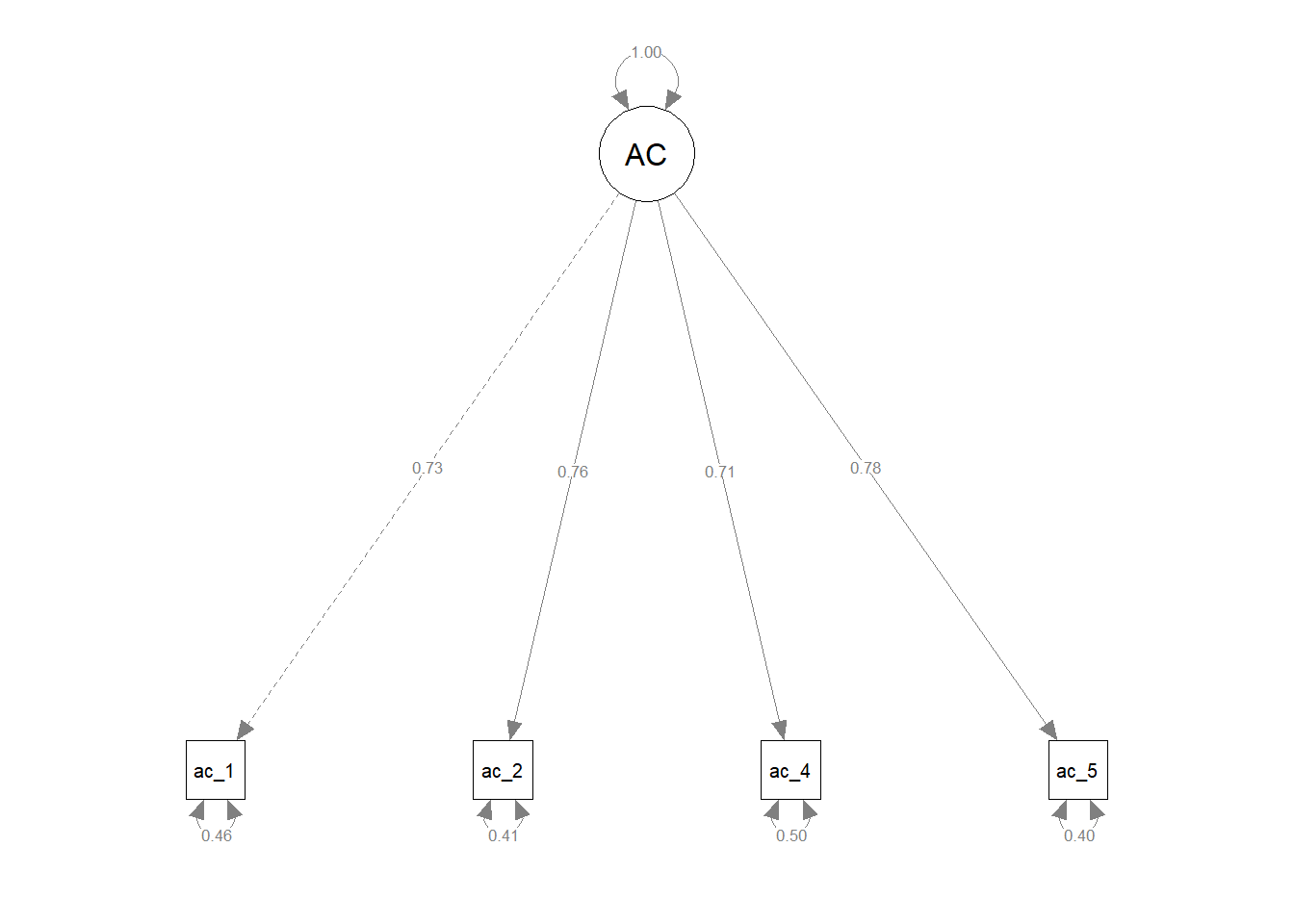

Let’s quickly review the model fit information, parameter estimates, average variance extracted (AVE), and composite reliability (CR) to see if they improved after removing item ac_3.

• Model fit indices. The model fit indices either remained about the same or improved after dropping item ac_3: chi-square test (\(\chi^{2}\) = 1.297, df = 2, p = .523), CFI (1.000), TLI (1.002), RMSEA (.000), and SRMR (.006).
• Parameter estimates. The parameter estimates also showed improvements after dropping item ac_3.
  • Factor loadings. After dropping item ac_3, all standardized factor loadings fell within the recommended range of .50 to .95, which indicated that they were acceptable. Specifically, the standardized factor loadings ranged from .709 to .776.
  • Error variances. The standardized error variances for the remaining four items (i.e., indicators) were all below the recommended cutoff of .50, which indicated that they were acceptable. Specifically, the standardized error variances ranged from .398 to .497.
  • Average variance extracted (AVE). After removing item ac_3, AVE increased from below the acceptable threshold of .50 to above the acceptable threshold. That is, the AVE estimate of .559 for the updated four-item feelings of acceptance measure was deemed acceptable.
  • Composite reliability (CR) After removing item ac_3, CR remained above the acceptable .70 threshold and improved relative to the previous estimate from when item ac_3 was still included. Thus, the CR estimate of .835 indicated acceptable reliability.
• Results write-up for the updated four-item measure of feelings of acceptance. As part of a new-employee onboarding survey administered 1-month after employees’ respective start dates, we assessed new employees on a five-item measure of feelings of acceptance. As noted above, we estimated a confirmatory factor analysis (CFA) model using the maximum likelihood (ML) estimator to evaluate the measurement structure for the five-item measure; however, item ac_3 showed a problematic standardized factor loading, standardized error variance, and misalignment between the item’s content and the conceptual definition for the associated measure. As a result, we re-specified and re-estimated the CFA model by removing item ac_3. In doing so, we found the following. The updated model showed acceptable fit to the data, as the chi-square test (\(\chi^{2}\) = 1.297, df = 2, p = .523), CFI (1.000), TLI (1.002), RMSEA (.000), and SRMR (.006) all met their respective cutoffs. The standardized factor loadings for the ac_1, ac_2, ac_4, and ac_5 items (.734, .765, .709, and .776, respectively) fell within the target .50-.95 range, thereby indicating they were all acceptable. The standardized error variances for items ac_1, ac_2, ac_4, and ac_5 (.461, .451, .497, and .398, respectively) all fell below the target threshold of .50, thereby indicating that it was unlikely that an unmodeled construct had an outsized influence on any of those four items. The average variance extracted (AVE) for the updated four-item measure was .559, which was above the conventional threshold of .50 and thus was deemed acceptable. Finally, the composite reliability (CR) reliability was .835, which exceeded the conventional threshold of .70 and thus was deemed acceptable. In sum, the measurement model for the updated four-item measure of feelings of acceptance showed acceptable fit to the data, and the parameter estimates, AVE, and CR were acceptable; however, when evaluating the parameter estimates, the standardized factor loading and standardized error variance for item ac_3 were both unacceptable. Thus, this four-item specification of the one-factor CFA model will be retained moving forward.

57.2.4.2 Estimate Just-Identified One-Factor Model

In the previous section, we evaluated the measurement structure for a four-item measure of feelings of acceptance, which resulted in an over-identified model (df > 0). In this section, we will review what happens when we specify a just-identified measurement model (df = 0).

For this example, we will evaluate the measurement model for the three-item measure of role clarity. As you can see below, we specified the three role clarity items as loading onto a latent factor for role clarity: RC =~ rc_1 + rc_2 + rc_3.

# Specify one-factor CFA model & assign to object
cfa_mod <- "
RC =~ rc_1 + rc_2 + rc_3
"

# Estimate one-factor CFA model & assign to fitted model object
cfa_fit <- cfa(cfa_mod,      # name of specified model object
               data=df)      # name of data frame object

# Print summary of model results
summary(cfa_fit,             # name of fitted model object
        fit.measures=TRUE,   # request model fit indices
        standardized=TRUE)   # request standardized estimates

## lavaan 0.6.15 ended normally after 17 iterations
## 
##   Estimator                                         ML
##   Optimization method                           NLMINB
##   Number of model parameters                         6
## 
##   Number of observations                           654
## 
## Model Test User Model:
##                                                       
##   Test statistic                                 0.000
##   Degrees of freedom                                 0
## 
## Model Test Baseline Model:
## 
##   Test statistic                               940.146
##   Degrees of freedom                                 3
##   P-value                                        0.000
## 
## User Model versus Baseline Model:
## 
##   Comparative Fit Index (CFI)                    1.000
##   Tucker-Lewis Index (TLI)                       1.000
## 
## Loglikelihood and Information Criteria:
## 
##   Loglikelihood user model (H0)              -2902.122
##   Loglikelihood unrestricted model (H1)      -2902.122
##                                                       
##   Akaike (AIC)                                5816.243
##   Bayesian (BIC)                              5843.142
##   Sample-size adjusted Bayesian (SABIC)       5824.092
## 
## Root Mean Square Error of Approximation:
## 
##   RMSEA                                          0.000
##   90 Percent confidence interval - lower         0.000
##   90 Percent confidence interval - upper         0.000
##   P-value H_0: RMSEA <= 0.050                       NA
##   P-value H_0: RMSEA >= 0.080                       NA
## 
## Standardized Root Mean Square Residual:
## 
##   SRMR                                           0.000
## 
## Parameter Estimates:
## 
##   Standard errors                             Standard
##   Information                                 Expected
##   Information saturated (h1) model          Structured
## 
## Latent Variables:
##                    Estimate  Std.Err  z-value  P(>|z|)   Std.lv  Std.all
##   RC =~                                                                 
##     rc_1              1.000                               1.157    0.847
##     rc_2              0.967    0.044   21.977    0.000    1.119    0.812
##     rc_3              0.924    0.042   22.107    0.000    1.070    0.819
## 
## Variances:
##                    Estimate  Std.Err  z-value  P(>|z|)   Std.lv  Std.all
##    .rc_1              0.527    0.051   10.279    0.000    0.527    0.282
##    .rc_2              0.646    0.053   12.142    0.000    0.646    0.340
##    .rc_3              0.560    0.048   11.793    0.000    0.560    0.329
##     RC                1.340    0.108   12.448    0.000    1.000    1.000

# Estimate average variance extracted (AVE)
AVE(cfa_fit)

##    RC 
## 0.683

# Estimate composite/construct reliability (CR)
compRelSEM(cfa_fit)

##    RC 
## 0.866

When reviewing the model output, note that the degrees of freedom (df) is equal to zero, which indicates that the model is just-identified. When a model is just-identified, our go-to model fit indices (chi-square test, CFI, TLI, RMSEA, SRMR) become irrelevant because the model fits the data perfectly from the viewpoint of those indices. The parameter estimates, however, can be estimated as usual. Similarly, the average variance extracted (AVE) and composite reliability (CR) can also be interpreted meaningfully. Please refer to the previous section for guidance on how to interpret the parameter, AVE, and CR estimates.

We can also visualize the CFA model as a path diagram for a just-identified model, just like we did with an over-identified model.

# Visualize the measurement model
semPaths(cfa_fit,         # name of fitted model object 
         what="std",      # display standardized parameter estimates
         weighted=FALSE,  # do not weight plot features
         nCharNodes=0)    # do not abbreviate names

57.2.5 Estimate Multi-Factor CFA Models

In the previous sections, we explored how to specify and estimate one-factor CFA models, or in other words, models with a single latent factor and all indicators loading onto that factor. In this section, we will learn how to specify multi-factor CFA models, which are models with two or more latent factors; specifically, we will focus on over-identified multi-factor CFA models. Multi-factor models are useful for determining whether theoretically distinguishable constructs are empirically distinguishable.

The new-employee onboarding survey data includes responses to three multi-item measures of new-employee adjustment into the organization: feelings of acceptance, role clarity, and task mastery. We modeled feelings of acceptance and role clarity as one-factor models in the previous sections, and in this section we’re going to specify a three-factor model with three latent factors corresponding to feelings of acceptance, role clarity, and task mastery and each measure’s items loading on their respective latent factor. In doing so, we can determine whether a three-factor model fits the data acceptably.

For more in-depth guidance on how to specify and evaluate a CFA model, please refer back to this section.

When we specify a multi-factor model, we simply repeat the process we used for a one-factor model. That is, in this three-factor model example, we will specify three latent factors. By default, the cfa function will freely estimate the covariance parameters between the three latent factors, constrain the first indicator for each latent factor to 1, and constrain the covariance parameters between the indicator error variance components to zero. Because we will learn how to compare nested models in the following section, let’s name the specified model object cfa_mod3 and the fitted model object cfa_fit_3 to communicate that we are evaluating a three-factor model. Everything else is specified in the same manner as the one-factor models from the previous sections.

# Specify three-factor CFA model & assign to object
cfa_mod_3 <- "
AC =~ ac_1 + ac_2 + ac_3 + ac_4 + ac_5
RC =~ rc_1 + rc_2 + rc_3
TM =~ tm_1 + tm_2 + tm_3 + tm_4
"

# Estimate three-factor CFA model & assign to fitted model object
cfa_fit_3 <- cfa(cfa_mod_3,  # name of specified model object
                 data=df)    # name of data frame object

# Print summary of model results
summary(cfa_fit_3,           # name of fitted model object
        fit.measures=TRUE,   # request model fit indices
        standardized=TRUE)   # request standardized estimates

## lavaan 0.6.15 ended normally after 33 iterations
## 
##   Estimator                                         ML
##   Optimization method                           NLMINB
##   Number of model parameters                        27
## 
##   Number of observations                           654
## 
## Model Test User Model:
##                                                       
##   Test statistic                               295.932
##   Degrees of freedom                                51
##   P-value (Chi-square)                           0.000
## 
## Model Test Baseline Model:
## 
##   Test statistic                              3312.955
##   Degrees of freedom                                66
##   P-value                                        0.000
## 
## User Model versus Baseline Model:
## 
##   Comparative Fit Index (CFI)                    0.925
##   Tucker-Lewis Index (TLI)                       0.902
## 
## Loglikelihood and Information Criteria:
## 
##   Loglikelihood user model (H0)             -12142.193
##   Loglikelihood unrestricted model (H1)     -11994.227
##                                                       
##   Akaike (AIC)                               24338.386
##   Bayesian (BIC)                             24459.430
##   Sample-size adjusted Bayesian (SABIC)      24373.705
## 
## Root Mean Square Error of Approximation:
## 
##   RMSEA                                          0.086
##   90 Percent confidence interval - lower         0.076
##   90 Percent confidence interval - upper         0.095
##   P-value H_0: RMSEA <= 0.050                    0.000
##   P-value H_0: RMSEA >= 0.080                    0.846
## 
## Standardized Root Mean Square Residual:
## 
##   SRMR                                           0.094
## 
## Parameter Estimates:
## 
##   Standard errors                             Standard
##   Information                                 Expected
##   Information saturated (h1) model          Structured
## 
## Latent Variables:
##                    Estimate  Std.Err  z-value  P(>|z|)   Std.lv  Std.all
##   AC =~                                                                 
##     ac_1              1.000                               0.945    0.734
##     ac_2              1.044    0.060   17.529    0.000    0.986    0.772
##     ac_3              0.272    0.063    4.345    0.000    0.257    0.186
##     ac_4              0.938    0.058   16.261    0.000    0.886    0.706
##     ac_5              1.100    0.063   17.473    0.000    1.040    0.768
##   RC =~                                                                 
##     rc_1              1.000                               1.156    0.846
##     rc_2              0.970    0.044   22.121    0.000    1.122    0.814
##     rc_3              0.925    0.042   22.217    0.000    1.069    0.819
##   TM =~                                                                 
##     tm_1              1.000                               1.160    0.757
##     tm_2              0.951    0.053   17.811    0.000    1.103    0.746
##     tm_3              0.963    0.053   18.112    0.000    1.117    0.760
##     tm_4              0.988    0.054   18.458    0.000    1.145    0.777
## 
## Covariances:
##                    Estimate  Std.Err  z-value  P(>|z|)   Std.lv  Std.all
##   AC ~~                                                                 
##     RC                0.271    0.053    5.151    0.000    0.248    0.248
##     TM                0.288    0.054    5.325    0.000    0.263    0.263
##   RC ~~                                                                 
##     TM                0.241    0.063    3.840    0.000    0.180    0.180
## 
## Variances:
##                    Estimate  Std.Err  z-value  P(>|z|)   Std.lv  Std.all
##    .ac_1              0.764    0.055   13.861    0.000    0.764    0.461
##    .ac_2              0.661    0.052   12.733    0.000    0.661    0.404
##    .ac_3              1.858    0.103   17.959    0.000    1.858    0.966
##    .ac_4              0.792    0.055   14.522    0.000    0.792    0.502
##    .ac_5              0.750    0.058   12.847    0.000    0.750    0.410
##    .rc_1              0.530    0.051   10.449    0.000    0.530    0.284
##    .rc_2              0.641    0.053   12.155    0.000    0.641    0.338
##    .rc_3              0.562    0.047   11.918    0.000    0.562    0.330
##    .tm_1              1.001    0.074   13.528    0.000    1.001    0.427
##    .tm_2              0.970    0.070   13.839    0.000    0.970    0.444
##    .tm_3              0.913    0.068   13.446    0.000    0.913    0.423
##    .tm_4              0.861    0.067   12.901    0.000    0.861    0.396
##     AC                0.893    0.089   10.068    0.000    1.000    1.000
##     RC                1.337    0.107   12.461    0.000    1.000    1.000
##     TM                1.345    0.127   10.572    0.000    1.000    1.000

# Estimate average variance extracted (AVE)
AVE(cfa_fit_3)

##    AC    RC    TM 
## 0.440 0.683 0.578

# Estimate composite/construct reliability (CR)
compRelSEM(cfa_fit_3)

##    AC    RC    TM 
## 0.788 0.866 0.845

# Visualize the measurement model
semPaths(cfa_fit_3,       # name of fitted model object 
         what="std",      # display standardized parameter estimates
         weighted=FALSE,  # do not weight plot features
         nCharNodes=0)    # do not abbreviate names

Evaluating model fit. Now that we have the summary of our model results, we will begin by evaluating key pieces of the model fit information provided in the output.

• Estimator. The function defaulted to using the maximum likelihood (ML) model estimator. When there are deviations from multivariate normality or categorical variables, the function may switch to another estimator.
• Number of parameters. Twenty-five parameters were estimated, which as we will see later correspond to factor loadings and (error) variance components.
• Number of observations. Our effective sample size is 654. Had there been missing data on the observed variables, this portion of the output would have indicated how many of the observations were retained for the analysis given the missing data. How missing data are handled during estimation will depend on the type of missing data approach we apply, which is covered in more default in the section called Estimating Models with Missing Data. By default, the cfa function applies listwise deletion in the presence of missing data.
• Chi-square test. The chi-square (\(\chi^{2}\)) test assesses whether the model fits the data adequately, where a statistically significant \(\chi^{2}\) value (e.g., p \(<\) .05) indicates that the model does not fit the data well and a nonsignificant chi-square value (e.g., p \(\ge\) .05) indicates that the model fits the data reasonably well (Bagozzi and Yi 1988). The null hypothesis for the \(\chi^{2}\) test is that the model fits the data perfectly, and thus failing to reject the null model provides some confidence that the model fits the data reasonably close to perfectly. Of note, the \(\chi^{2}\) test is sensitive to sample size and non-normal variable distributions. For this model, we find the \(\chi^{2}\) test in the output section labeled Model Test User Model. Because the p-value is less than .05, we reject the null hypothesis that the mode fits the data perfectly and thus conclude that the model does not fit the data acceptably (\(\chi^{2}\) = 295.932, df = 51, p < .001), at least according to this test. Finally, note that because the model’s degrees of freedom (i.e., 51) is greater than zero, we can conclude that the model is over-identified.
• Comparative fit index (CFI). As the name implies, the comparative fit index (CFI) is a type of comparative (or incremental) fit index, which means that CFI compares our estimated model to a baseline model, which is commonly referred to as the null or independence model. CFI is generally less sensitive to sample size than the chi-square (\(\chi^{2}\)) test. A CFI value greater than or equal to .95 generally indicates good model fit to the data, although some might relax that cutoff to .90. For this model, CFI is equal to .925, which is above the .90 relaxed cutoff but below the .95 stringent cutoff. Based on this index, we can include that the model shows marginal fit to the data.
• Tucker-Lewis index (TLI). Like CFI, Tucker-Lewis index (TLI) is another type of comparative (or incremental) fit index. TLI is generally less sensitive to sample size than the chi-square test and tends to work well with smaller sample sizes; however, as Hu and Bentler (1999) noted, TLI may be not be the best choice for smaller sample sizes (e.g., N \(<\) 250). A TLI value greater than or equal to .95 generally indicates good model fit to the data, although like CFI, some might relax that cutoff to .90. For this model, TLI is equal to .902, which is above the .90 relaxed cutoff but below the .95 stringent cutoff. Based on this index, we can include that the model shows marginal fit to the data.
• Loglikelihood and Information Criteria. The section labeled Loglikelihood and Information Criteria contains model fit indices that are not directly interpretable on their own (e.g., loglikelihood, AIC, BIC). Rather, they become more relevant when we wish to compare the fit of two or more non-nested models. Given that, we will will ignore this section in this tutorial.
• Root mean square error of approximation (RMSEA). The root mean square error of approximation (RMSEA) is an absolute fit index that penalizes model complexity (e.g., models with a larger number of estimated parameters) and thus effectively rewards models that are more parsimonious. RMSEA values tend to upwardly biased when the model degrees of freedom are fewer (i.e., when the model is closer to being just-identified); further, Hu and Bentler (1999) noted that RMSEA may not be the best choice for smaller sample sizes (e.g., N \(<\) 250). In general, an RMSEA value that is less than or equal to .06 indicates good model fit to the data, although some relax that cutoff to .08 or even .10. For this model, RMSEA is equal to .086, which is above the .06 stringent cutoff but below the more relaxed .10 cutoff. This indicates that the model fits the data marginally well.
• Standardized root mean square residual. Like the RMSEA, the standardized root mean square residual (SRMR) is an example of an absolute fit index. An SRMR value that is less than or equal to .06 generally indicates good fit to the data, although some relax that cutoff to .08. For this model, SRMR is equal to .094, which indicates that the model does not fit the data acceptably.

In sum, the chi-square (\(\chi^{2}\)) test indicated that the model did not fit the data acceptably, but as noted above, this test is sensitive to sample size and non-normality. While the CFI, TLI, and RMSEA estimates did not meet their respective stringent cutoffs, they did meet their more relaxed cutoffs, indicating that the model fit to the data was marginal but showed room for improvement. The SRMR estimate, however, was well above the .06 stringent cutoff and the .08 relaxed cutoff, indicating that the model did not fit the data acceptably. Although not terrible, these less than optimal model fit index estimates suggest that perhaps our model was misspecified in some way. We will evaluate the parameter estimates next to see if we can identify any problematic parameter estimates that may explain the lower-than-desired model fit index estimates that we observed.

Evaluating parameter estimates. As noted above, our model fit information indicated that the model marginally fit the data for the most part, so we can feel reasonably comfortable interpreting and evaluating the parameter estimates. By default, the cfa function provides unstandardized parameter estimates, but if you recall, we also requested standardized parameter estimates. In the output, the unstandardized parameter estimates fall under the column titled Estimates, whereas the standardized factor loadings we’re interested in fall under the column titled Std.all.

• Factor loadings. The output section labeled Latent Variables contains our factor loadings. For this model, the loadings represent the effects of the latent factors for feelings of acceptance, role clarity, and task mastery on the their respective items. By default, the cfa function constrains the factor loading associated with the first indicator of each latent factor to 1 for model estimation purposes. Note, however, that there are still substantive standardized factor loadings for those first indicators, but they lack standard error (SE), z-value, and p-value estimates. We can still evaluate those standardized factor loadings, though. First, regarding the feelings of acceptance (AC) latent factor, with the exception of the ac_3 item, all standardized factor loadings (.706-.772) fell within Bagozzi and Yi’s (1988) recommended range of .50-.95; however, the standardized factor loading for the ac_3 item was .186, which was far below the lower limit of the recommended range. Thus, the AC latent factor showed a weak association with the ac_3 item, and we’ll consider this to be an unacceptable indicator of the AC latent factor. Let’s review the item’s content and the conceptual definition for feelings of acceptance, which appears in the Initial Steps section. The item content is: “My colleagues and I feel confident in our ability to complete work.” And the conceptual definition is: “the extent to which an individual feels welcomed and socially accepted at work.” Clearly, this item’s content does not fit within the bounds of the conceptual definition; in fact, it looks as though it may be more closely related to the conceptual definition for the task mastery construct. Given the very low standardized factor loading the and item content lack of alignment with the conceptual definition, we will drop this item whenever we re-estimate the model. Note: Had this standardized factor loading been just below .50 or just above .95, we would have looked at the item content to determine whether it fit with the conceptual definition, and if it had aligned with the conceptual definition, we would have likely retained the item. Second, regarding the role clarity (RC) latent factor, all standardized factor loadings (.814-.846) fell within recommended range of .50-.95. Third, regarding the task mastery (TM) latent factor, all standardized factor loadings (.746-.777) fell within recommended range of .50-.95.
• Covariances. The output section labeled Covariances contains the pairwise covariance estimates for the three latent factors. As was the case with the factor loadings, we can view the standardized and unstandardized parameter estimates, where the standardized covariances can be interpreted as correlations. First, the correlation between AC and RC was .248 and statistically significant (p < .001), and can be considered small-to-medium-sized in terms of practical significance. Second, the correlation between AC and TM was .263 and statistically significant (p < .001), and can also be considered small-to-medium-sized in terms of practical significance. Finally, the correlation between RC and TM was .180 and statistically significant (p < .001), and can be considered small-sized in terms of practical significance.
• Variances The output section labeled Variances contains the (error) variance estimates for each observed indicator (i.e., item) of the latent factor and for the latent factor itself. As was the case with the factor loadings, we can view the standardized and unstandardized parameter estimates.
  • Error variances for indicators. The estimates associated with the four indicator variables represent the error variances. Sometimes these are referred to as residual variances, disturbance terms, or uniquenesses. The standardized error variances ranged from .284 to .966, which can be interpreted as proportions of the variance not explained by the latent factor. For example, the latent factor AC failed to explain 46.1% of the variance in the indicator ac_1, which is acceptable; this suggests that 53.9% (100% - 46.1%) of the variance in indicator ac_1 was explained by the latent factor AC. With the exceptions of the ac_3 item’s error variance (.996) and the ac_4 item’s error variance (.502), the indicator error variances were less than the recommended .50 threshold, which means that unmodeled constructs did not likely have a notable impact on the vast majority of the indicators. The standardized error variance associated with the ac_3 item was well above the .50 threshold and its value indicates that the AC latent factor fails to explain 96.6% of the variance in that item, which is quite bad. Given the low standardized factor loading above, the item content’s misalignment with the conceptual definition for the construct, and this very high standardized error variance, we should feel confident that it is appropriate to remove indicator ac_3 prior to re-estimating the model. In contrast, the standardized error variance for the ac_4 item was just above the .50 recommended cutoff, and if we check the item’s content (“My colleagues listen thoughtfully to my ideas.”) and the construct’s conceptual definition (“the extent to which an individual feels welcomed and socially accepted at work”), we see that the item fits within the conceptual definition boundaries; thus, we should retain the ac_4 item when re-estimating the model.
  • Variance of the latent factors. The variance estimate for the latent factor provides can provide an indication of the latent factors’ level variability; however, its value depends on the scaling of factor loadings, and generally it is not a point of interest when evaluating CFA models. By default, the standardized variance for the latent factor will be equal to 1.000, and thus if we wished to evaluate the latent factor variance, we would interpret the unstandardized variance in this instance.

Average variance extracted (AVE). The AVE estimates for feelings of acceptance (AC), role clarity (RC), and task mastery (TM) were .440, .683, and .845, respectively. The AVE estimates associated with the the RC and TM latent factors exceeded the conventional threshold (\(\ge\) .50), and thus, we can conclude that those AVE estimates were acceptable. In contrast, the AVE estimate associated with the AC latent factor fell below the .50 cutoff. This lower-than-desired AVE estimate may be the result of the problematic parameter estimates associated with the ac_3 item, as noted above.

Composite reliability (CR). The CR estimates for feelings of acceptance (AC), role clarity (RC), and task mastery (TM) were .788, .866, and .845, respectively, which exceeded the conventional threshold for acceptable reliability (\(\ge\) .70) as well as the more relaxed “questionable” threshold (\(\ge\) .60). We can conclude that three latent factors demonstrated acceptable internal consistency reliability; with that being said, we may be able to improve the CR for the AC latent factor by dropping the problematic ac_3 item.

Results write-up for the initial three-factor model. As part of a new-employee onboarding survey administered 1-month after employees’ respective start dates, we assessed new employees on three multi-item measures targeting feelings of acceptance, role clarity, and task mastery. Using confirmatory factor analysis (CFA), we evaluated the measurement structure of the three multi-item measures, where each item served as an indicator for its respective latent factor; we did not allow indicator error variances to covary (i.e., the associations were constrained to zero) and, by default, the first indicator for each latent factor (i.e., ac_1) was constrained to 1 for estimation purposes and the latent-factor covariances were estimated freely. The three-factor model was estimated using the maximum likelihood (ML) estimator and a sample size of 654 new employees. Missing data were not a concern. We evaluated the model’s fit to the data using the chi-square (\(\chi^{2}\)) test, CFI, TLI, RMSEA, and SRMR model fit indices. The \(\chi^{2}\) test indicated that the model fit the data worse than a perfectly fitting model (\(\chi^{2}\) = 295.932, df = 51, p < .000). Further, the CFI and TLI estimates were .925 and .902, respectively, which did not exceed the more stringent threshold of .95 but did exceed the more relaxed threshold of .90, thereby indicating that model showed marginal fit to the data. Similarly, the RMSEA estimate was .086, which was not below the more stringent threshold of .06 but was below the more relaxed threshold of .10, thereby indicating that model showed marginal fit to the data. The SRMR estimate was .094, which was about both the stringent threshold of .06 and the relaxed threshold of .08, thereby indicating unacceptable model fit to the data. Collectively, the model fit information indicated that model showed mostly marginal fit to the data, which indicated the model may have been misspecified. Excluding the ac_3 item, the standardized factor loadings ranged from .706 to .846, which means that those item’s standardize factor loadings fell well within the acceptable range of .50-.95; however, the standardized factor loading for the ac_3 item was .186, which was a great deal outside the acceptable range. Regarding the standardized covariance estimates, the correlation between feelings of acceptance and role clarity latent factors was .248, statistically significant (p < .001), and small-to-medium in terms of practical significance; the correlation between feelings of acceptance and task mastery latent factors was .263, statistically significant (p < .001), and small-to-medium in terms of practical significance; and the correlation between role clarity and task mastery latent factors was .180, statistically significant (p < .001), and small in terms of practical significance. The standardized error variances ranged from .284 to .966, which can be interpreted as proportions of the variance not explained by the latent factor. With the exceptions of the ac_3 item’s error variance (.966) and the ac_4 item’s error variance (.502), the indicator error variances were less than the recommended .50 threshold, which means that unmodeled constructs did not likely have a notable impact on the vast majority of the indicators. The standardized error variance associated with the ac_3 item was well above the .50 threshold and its value indicates that the AC latent factor fails to explain 96.6% of the variance in that item, which is unacceptable. Given the ac_3 item’s unacceptably low standardized factor loading and unacceptably high standardized error variance, we reviewed the item’s content (“My colleagues and I feel confident in our ability to complete work.”) and the feelings of acceptance construct’s conceptual definition (“the extent to which an individual feels welcomed and socially accepted at work”). Because the item’s content does not align with the conceptual definition and because of the unacceptable standardized factor loading and error variance, we decided to drop item ac_3 prior to re-estimating the model. In contrast, the standardized error variance for the ac_4 item was just above the .50 recommended cutoff, and after reviewing the item’s content (“My colleagues listen thoughtfully to my ideas.”) and the construct’s conceptual definition, we determined that the item fits within the conceptual definition boundaries; thus, we decided to retain the ac_4 item when re-estimating the model. The average variance extracted (AVE) estimates for feelings of acceptance, role clarity, and task mastery were .440, .683, and .578, respectively. The AVE estimates associated with the the RC and TM latent factors exceeded the conventional threshold (\(\ge\) .50), and thus, we can conclude that those factors showed acceptable levels of AVE. In contrast, the AVE estimate associated with the AC latent factor fell below the .50 cutoff; this unacceptable AVE estimate may be the result of the problematic parameter estimates associated with the ac_3 item that we noted above. The composite reliability (CR) estimates for feelings of acceptance, role clarity, and task mastery were .788, .866, and .845, respectively, which exceeded the conventional threshold of .70 and thus were deemed acceptable. In sum, the three-factor measurement model showed marginal fit to the data, and CR estimates were acceptable; however, when evaluating the parameter estimates, the standardized factor loading and standardized error variance for item ac_3 were both unacceptable; further, while the AVE estimates associated with the role clarity (RC) and task mastery (TM) latent factors were acceptable, the AVE associated with the feelings of acceptance (AC) latent factor was unacceptable, which may be attributable to the low standardized factor loading associated with item ac_3.

Removing the problematic item and re-estimating the three-factor CFA model. Given the problematic nature of the ac_3 item shown above, we will re-estimate the three-factor CFA model without the ac_3 item.

# Re-specify three-factor CFA model without ac_3 item & assign to object
cfa_mod_3 <- "
AC =~ ac_1 + ac_2 + ac_4 + ac_5
RC =~ rc_1 + rc_2 + rc_3
TM =~ tm_1 + tm_2 + tm_3 + tm_4
"

# Re-estimate three-factor CFA model without ac_3 item & assign to fitted model object
cfa_fit_3 <- cfa(cfa_mod_3,  # name of specified model object
                 data=df)    # name of data frame object

# Print summary of model results
summary(cfa_fit_3,           # name of fitted model object
        fit.measures=TRUE,   # request model fit indices
        standardized=TRUE)   # request standardized estimates

## lavaan 0.6.15 ended normally after 31 iterations
## 
##   Estimator                                         ML
##   Optimization method                           NLMINB
##   Number of model parameters                        25
## 
##   Number of observations                           654
## 
## Model Test User Model:
##                                                       
##   Test statistic                               113.309
##   Degrees of freedom                                41
##   P-value (Chi-square)                           0.000
## 
## Model Test Baseline Model:
## 
##   Test statistic                              3111.443
##   Degrees of freedom                                55
##   P-value                                        0.000
## 
## User Model versus Baseline Model:
## 
##   Comparative Fit Index (CFI)                    0.976
##   Tucker-Lewis Index (TLI)                       0.968
## 
## Loglikelihood and Information Criteria:
## 
##   Loglikelihood user model (H0)             -11009.696
##   Loglikelihood unrestricted model (H1)     -10953.042
##                                                       
##   Akaike (AIC)                               22069.392
##   Bayesian (BIC)                             22181.470
##   Sample-size adjusted Bayesian (SABIC)      22102.095
## 
## Root Mean Square Error of Approximation:
## 
##   RMSEA                                          0.052
##   90 Percent confidence interval - lower         0.041
##   90 Percent confidence interval - upper         0.063
##   P-value H_0: RMSEA <= 0.050                    0.372
##   P-value H_0: RMSEA >= 0.080                    0.000
## 
## Standardized Root Mean Square Residual:
## 
##   SRMR                                           0.032
## 
## Parameter Estimates:
## 
##   Standard errors                             Standard
##   Information                                 Expected
##   Information saturated (h1) model          Structured
## 
## Latent Variables:
##                    Estimate  Std.Err  z-value  P(>|z|)   Std.lv  Std.all
##   AC =~                                                                 
##     ac_1              1.000                               0.946    0.735
##     ac_2              1.041    0.059   17.496    0.000    0.984    0.770
##     ac_4              0.940    0.058   16.301    0.000    0.889    0.708
##     ac_5              1.105    0.063   17.530    0.000    1.045    0.772
##   RC =~                                                                 
##     rc_1              1.000                               1.156    0.846
##     rc_2              0.970    0.044   22.118    0.000    1.122    0.814
##     rc_3              0.925    0.042   22.213    0.000    1.069    0.819
##   TM =~                                                                 
##     tm_1              1.000                               1.159    0.757
##     tm_2              0.951    0.053   17.801    0.000    1.103    0.746
##     tm_3              0.964    0.053   18.103    0.000    1.117    0.760
##     tm_4              0.988    0.054   18.445    0.000    1.145    0.777
## 
## Covariances:
##                    Estimate  Std.Err  z-value  P(>|z|)   Std.lv  Std.all
##   AC ~~                                                                 
##     RC                0.264    0.053    5.022    0.000    0.241    0.241
##     TM                0.267    0.054    4.975    0.000    0.244    0.244
##   RC ~~                                                                 
##     TM                0.241    0.063    3.838    0.000    0.180    0.180
## 
## Variances:
##                    Estimate  Std.Err  z-value  P(>|z|)   Std.lv  Std.all
##    .ac_1              0.763    0.055   13.832    0.000    0.763    0.460
##    .ac_2              0.665    0.052   12.770    0.000    0.665    0.407
##    .ac_4              0.788    0.054   14.466    0.000    0.788    0.499
##    .ac_5              0.740    0.058   12.699    0.000    0.740    0.404
##    .rc_1              0.530    0.051   10.446    0.000    0.530    0.284
##    .rc_2              0.641    0.053   12.152    0.000    0.641    0.338
##    .rc_3              0.562    0.047   11.916    0.000    0.562    0.330
##    .tm_1              1.002    0.074   13.528    0.000    1.002    0.427
##    .tm_2              0.969    0.070   13.830    0.000    0.969    0.444
##    .tm_3              0.913    0.068   13.433    0.000    0.913    0.422
##    .tm_4              0.861    0.067   12.892    0.000    0.861    0.396
##     AC                0.894    0.089   10.072    0.000    1.000    1.000
##     RC                1.337    0.107   12.461    0.000    1.000    1.000
##     TM                1.344    0.127   10.565    0.000    1.000    1.000

# Estimate average variance extracted (AVE)
AVE(cfa_fit_3)

##    AC    RC    TM 
## 0.559 0.683 0.578

# Estimate composite/construct reliability (CR)
compRelSEM(cfa_fit_3)

##    AC    RC    TM 
## 0.835 0.866 0.845

# Visualize the measurement model
semPaths(cfa_fit_3,       # name of fitted model object 
         what="std",      # display standardized parameter estimates
         weighted=FALSE,  # do not weight plot features
         nCharNodes=0)    # do not abbreviate names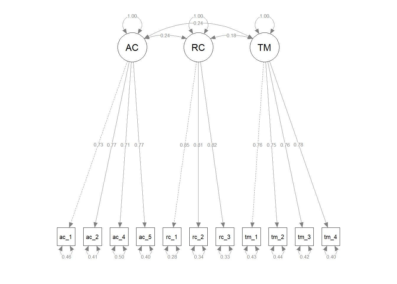

Let’s quickly review the model fit information, parameter estimates, average variance extracted (AVE), and composite reliability (CR) to see if they improved after removing item ac_3.

• Model fit indices. With the exception of the chi-square test, model fit indices improved after dropping item ac_3: chi-square test (\(\chi^{2}\) = 113.309, df = 41, p < .001), CFI (.976), TLI (.968), RMSEA (.052), and SRMR (.032). Specifically, CFI, TLI, RMSEA, and SRMR estimates all met their more stringent cutoffs and thus indicated the model fit the data acceptably.
• Parameter estimates. The parameter estimates also showed improvements after dropping item ac_3.
  • Factor loadings. After dropping item ac_3, all standardized factor loadings fell within the recommended range of .50 to .95, which indicated that they were acceptable. Specifically, the standardized factor loadings ranged from .708 to .846.
  • Covariances. After dropping item ac_3, all standardized covariances remained statistically significant, and their practical significance levels remained similar to those observed in the initial model that included item ac_3. Specifically, the correlations were .241 (p < .001), .244 (p < .001), and .180 (p < .001) for AC in relation to RC, AC in relation to TM, and RC in relation to TM, respectively.
  • Error variances. After dropping item ac_3, the standardized error variances for the items (i.e., indicators) were all below the recommended cutoff of .50, which indicated that they were acceptable. Specifically, the standardized error variances ranged from .284 to .499.
  • Average variance extracted (AVE). After removing item ac_3, AVE estimate associated with the AC latent factor increased from below the acceptable threshold of .50 to above the acceptable threshold. That is, the AVE estimate of .559 for the updated four-item feelings of acceptance measure was deemed acceptable. Further, the AVE estimates associated with the RC and TM latent factors remained above the .50 threshold. Specifically, the AVE estimates associated with the RC and TM latent factors were .683 and .578, respectively.
  • Composite reliability (CR) After removing item ac_3, CR estimates remained above the acceptable .70 threshold and, for the AC latent factor, improved relative to the previous estimate from when item ac_3 was still included. The CR estimates of .835 for AC, .866 for RC, and .845 for TM all indicated acceptable levels of internal consistency reliability.
• Results write-up for the updated three-factor CFA model. As part of a new-employee onboarding survey administered 1-month after employees’ respective start dates, we assessed new employees using three multi-item measures designed to measure feelings of acceptance, role clarity, and task mastery. As noted above, we estimated a three-factor confirmatory factor analysis (CFA) model using the maximum likelihood (ML) estimator to evaluate the measurement structure for the three multi-item measures; however, item ac_3 showed a problematic standardized factor loading, standardized error variance, and misalignment between the item’s content and the conceptual definition for the associated measure. As a result, we re-specified and re-estimated the CFA model by removing item ac_3. In doing so, we found the following. The updated model showed acceptable fit to the data according to CFI (.976), TLI (.968), RMSEA (.052), and SRMR (.032). The chi-square test (\(\chi^{2}\) = 113.309, df = 41, p < .001), however, indicated that the model did not fit the data well; that said, the chi-square test is sensitive to sample size. We concluded that in general the model showed acceptable fit to the data. Standardized factor loadings ranged from .708 to .846, which all fell well within the recommended .50-.95 acceptability range. The standardized error variances for items ranged from .284 to .499, and thus all fell below the target threshold of .50, thereby indicating that it was unlikely that an unmodeled construct had an outsized influence on any of those items. The average variance extracted (AVE) for feelings of acceptance, role clarity, and task mastery were .559, .683, and .578, respectively, which all exceeded the .50 cutoff; thus, all three latent factors showed acceptable AVE levels. Finally, the composite reliability (CR) estimates were .835 for feelings of acceptance, .866 for role clarity, and .845 for task mastery, and all indicated acceptable levels of internal consistency reliability. In sum, the updated three-factor measurement model in which the ac_3 item was removed showed acceptable fit to the data, acceptable parameter estimates, acceptable AVE estimates, and acceptable CR estimates. Thus, this specification of the three-factor CFA model will be retained moving forward.

57.2.6 Nested Model Comparisons

When evaluating measurement structures, there are variety of circumstances in which we might wish to compare nested models. A nested model has all the same parameter estimates of a full model but has additional parameter constraints in place; a nested model will have more degrees of freedom (df) than the full model, thereby indicating that the nested model is more parsimonious.

In this section, we will evaluate whether the updated and final three-factor model we estimated in the previous section, where the problematic ac_3 item was removed, fits significantly better than models with additional constraints. In general, our goal will be to retain the most parsimonious model that fits the data acceptably.

57.2.6.1 Two-Factor Model (Version a)

We’ll begin by specifying an alternative model where we load the items associated with the feelings of acceptance and role clarity measures onto a single factor that we’ll label AC_RC. We’ll keep the task mastery items loaded on a latent factor labeled TM. In this way, we’ve created a two-factor model, and we’ll name this model specification object (cfa_mod_2a).

# Specify two-factor CFA model & assign to object (version a)
cfa_mod_2a <- "
AC_RC =~ ac_1 + ac_2 + ac_4 + ac_5 + rc_1 + rc_2 + rc_3
TM =~ tm_1 + tm_2 + tm_3 + tm_4
"

# Estimate three-factor CFA model & assign to fitted model object
cfa_fit_2a <- cfa(cfa_mod_2a, # name of specified model object
                  data=df)    # name of data frame object    

At this point, you may be wondering: “How is the two-factor model (cfa_mod_2a) nested within the original three factor model (cfa_mod_3)?” That is, it may not look as though we applied any direct constraints to the three-factor model to result in the two-factor model. Perhaps the following alternative approach to specifying the two-factor model will clear up any confusion. Specifically, instead of collapsing the feelings of acceptance and role clarity items onto a single factor labeled AC_RC, we will retain the original three-factor model specification but add constraints to the model. First, we will set the covariance between the AC and RC latent factors to 1, which we can achieve by specifying: AC ~~ 1*RC. If you recall, the ~~ operator is used to specify covariances. Second, we will add the std.lv=TRUE argument to our cfa function to set all of the latent factor variances to 1 (i.e., standardized). Finally, because the AC and RC latent factors will be set to act as a single factor, we need to make sure that we constrain their respective covariances with TM to be equal, which we can achieve by specifying: AC ~~ cov*TM and RC ~~ cov*TM; note that the cov is an arbitrary constraint label that I’m applying, and you could name the constraint whatever you’d like so long as it is the same name across the two covariances and we follow the constraint name with the * operator.

# Alternative approach: Specify two-factor CFA model & assign to object (version a)
cfa_mod_2a <- "
AC =~ ac_1 + ac_2 + ac_3 + ac_4 + ac_5
RC =~ rc_1 + rc_2 + rc_3
TM =~ tm_1 + tm_2 + tm_3 + tm_4

# Constrain AC & RC covariance to 1
AC ~~ 1*RC

# Constrain covariances to be equal
AC ~~ cov*TM
RC ~~ cov*TM
"

# Estimate three-factor CFA model & assign to fitted model object
cfa_fit_2a <- cfa(cfa_mod_2a,  # name of specified model object
                  data=df,     # name of data frame object 
                  std.lv=TRUE) # constrain factor variances to 1   

Because specifying the alternative approach to the two-factor model is more time intensive, let’s revert back to the initial specification and then estimate the model.

# Specify two-factor CFA model & assign to object (version a)
cfa_mod_2a <- "
AC_RC =~ ac_1 + ac_2 + ac_4 + ac_5 + rc_1 + rc_2 + rc_3
TM =~ tm_1 + tm_2 + tm_3 + tm_4
"

# Estimate three-factor CFA model & assign to fitted model object
cfa_fit_2a <- cfa(cfa_mod_2a, # name of specified model object
                  data=df)    # name of data frame object    

# Print summary of model results
summary(cfa_fit_2a,           # name of fitted model object
        fit.measures=TRUE,    # request model fit indices
        standardized=TRUE)    # request standardized estimates

## lavaan 0.6.15 ended normally after 30 iterations
## 
##   Estimator                                         ML
##   Optimization method                           NLMINB
##   Number of model parameters                        23
## 
##   Number of observations                           654
## 
## Model Test User Model:
##                                                       
##   Test statistic                               994.577
##   Degrees of freedom                                43
##   P-value (Chi-square)                           0.000
## 
## Model Test Baseline Model:
## 
##   Test statistic                              3111.443
##   Degrees of freedom                                55
##   P-value                                        0.000
## 
## User Model versus Baseline Model:
## 
##   Comparative Fit Index (CFI)                    0.689
##   Tucker-Lewis Index (TLI)                       0.602
## 
## Loglikelihood and Information Criteria:
## 
##   Loglikelihood user model (H0)             -11450.330
##   Loglikelihood unrestricted model (H1)     -10953.042
##                                                       
##   Akaike (AIC)                               22946.660
##   Bayesian (BIC)                             23049.772
##   Sample-size adjusted Bayesian (SABIC)      22976.747
## 
## Root Mean Square Error of Approximation:
## 
##   RMSEA                                          0.184
##   90 Percent confidence interval - lower         0.174
##   90 Percent confidence interval - upper         0.194
##   P-value H_0: RMSEA <= 0.050                    0.000
##   P-value H_0: RMSEA >= 0.080                    1.000
## 
## Standardized Root Mean Square Residual:
## 
##   SRMR                                           0.137
## 
## Parameter Estimates:
## 
##   Standard errors                             Standard
##   Information                                 Expected
##   Information saturated (h1) model          Structured
## 
## Latent Variables:
##                    Estimate  Std.Err  z-value  P(>|z|)   Std.lv  Std.all
##   AC_RC =~                                                              
##     ac_1              1.000                               0.928    0.721
##     ac_2              1.059    0.062   17.181    0.000    0.983    0.769
##     ac_4              0.948    0.060   15.916    0.000    0.880    0.701
##     ac_5              1.110    0.065   17.056    0.000    1.030    0.761
##     rc_1              0.417    0.063    6.604    0.000    0.387    0.283
##     rc_2              0.429    0.064    6.742    0.000    0.398    0.289
##     rc_3              0.385    0.060    6.385    0.000    0.357    0.274
##   TM =~                                                                 
##     tm_1              1.000                               1.156    0.755
##     tm_2              0.952    0.054   17.737    0.000    1.101    0.745
##     tm_3              0.969    0.054   18.103    0.000    1.120    0.762
##     tm_4              0.991    0.054   18.411    0.000    1.146    0.778
## 
## Covariances:
##                    Estimate  Std.Err  z-value  P(>|z|)   Std.lv  Std.all
##   AC_RC ~~                                                              
##     TM                0.280    0.053    5.270    0.000    0.261    0.261
## 
## Variances:
##                    Estimate  Std.Err  z-value  P(>|z|)   Std.lv  Std.all
##    .ac_1              0.796    0.056   14.176    0.000    0.796    0.480
##    .ac_2              0.667    0.052   12.829    0.000    0.667    0.409
##    .ac_4              0.803    0.055   14.614    0.000    0.803    0.509
##    .ac_5              0.769    0.059   13.075    0.000    0.769    0.420
##    .rc_1              1.717    0.097   17.779    0.000    1.717    0.920
##    .rc_2              1.741    0.098   17.765    0.000    1.741    0.916
##    .rc_3              1.577    0.089   17.801    0.000    1.577    0.925
##    .tm_1              1.009    0.074   13.572    0.000    1.009    0.430
##    .tm_2              0.973    0.070   13.850    0.000    0.973    0.445
##    .tm_3              0.906    0.068   13.362    0.000    0.906    0.419
##    .tm_4              0.859    0.067   12.861    0.000    0.859    0.395
##     AC_RC             0.862    0.088    9.834    0.000    1.000    1.000
##     TM                1.337    0.127   10.530    0.000    1.000    1.000

# Visualize the measurement model
semPaths(cfa_fit_2a,      # name of fitted model object 
         what="std",      # display standardized parameter estimates
         weighted=FALSE,  # do not weight plot features
         nCharNodes=0)    # do not abbreviate names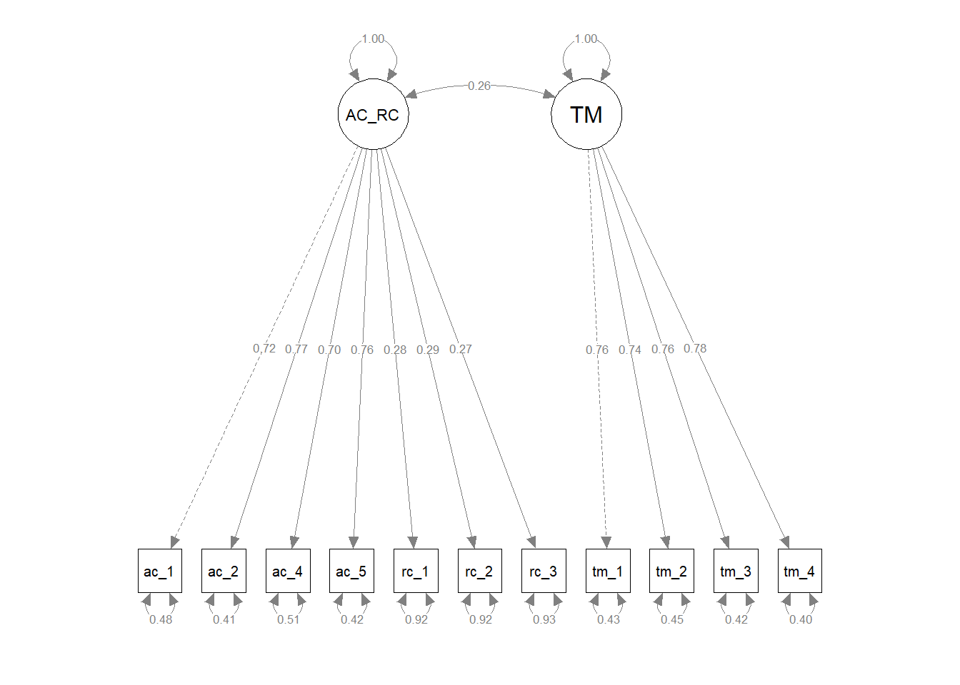

Just as we did with the three-factor model in the previous section, we would first evaluate the model fit, and if the model fit appears acceptable, then we would evaluate the parameter estimates. To save space, however, we will skip directly to comparing this version of the two-factor model to our original three-factor model, which I summarize in the table below.

Model	\(\chi^{2}\)	df	p	CFI	TLI	RMSEA	SRMR
3-Factor Model	113.309	41	< .001	.976	.968	.052	.032
2a-Factor Model	994.577	43	< .001	.689	.602	.184	.137

As you can see above, the first version (version a) of the two-factor model fits the data notably worse than the three-factor model, which suggests that the three-factor model is probably a better representation of the measurement structure.

As an additional test, we can perform a nested model comparison using the chi-square (\(\chi^{2}\)) difference test, which is also known as the log-likelihood (LL) test. To perform this test, we’ll apply the anova function from base R. As the first argument, we’ll insert the name of our three-factor model object (cfa_fit_3), and as the second argument, we’ll insert the name of our two-factor model object (cfa_fit_2a).

# Nested model comparison using chi-square difference test
anova(cfa_fit_3, cfa_fit_2a)

## 
## Chi-Squared Difference Test
## 
##            Df   AIC   BIC  Chisq Chisq diff   RMSEA Df diff            Pr(>Chisq)    
## cfa_fit_3  41 22069 22182 113.31                                                     
## cfa_fit_2a 43 22947 23050 994.58     881.27 0.81989       2 < 0.00000000000000022 ***
## ---
## Signif. codes:  0 '***' 0.001 '**' 0.01 '*' 0.05 '.' 0.1 ' ' 1

The chi-square difference test indicates that the first version of the two-factor model fits the data statistically significantly worse than the original three-factor model (\(\Delta \chi^{2}\) = 881.27, \(\Delta df\) = 2, \(p\) < .001). This corroborates what we saw with the direct comparison of model fit indices above.

Note: If your anova function output defaulted to scientific notation, you can “turn off” scientific notation using the following function. After running the options function below, you can re-run the anova function to get the output in traditional notation.

# Turn off scientific notation
options(scipen=9999)

57.2.6.2 Two-Factor Model (Version b)

We’ll now evaluate a second version of a two-factor model (version b). In this version, we’ll collapse latent factors RC and TM into a single latent factor and load their respective items on the single factor labeled RC_TM. We’ll specify the AC latent factor such that only the corresponding feelings of acceptance items load on it.

# Specify two-factor CFA model & assign to object (version b)
cfa_mod_2b <- "
AC =~ ac_1 + ac_2 + ac_4 + ac_5
RC_TM =~ rc_1 + rc_2 + rc_3 + tm_1 + tm_2 + tm_3 + tm_4
"

# Estimate three-factor CFA model & assign to fitted model object
cfa_fit_2b <- cfa(cfa_mod_2b, # name of specified model object
                  data=df)    # name of data frame object

# Print summary of model results
summary(cfa_fit_2b,          # name of fitted model object
        fit.measures=TRUE,   # request model fit indices
        standardized=TRUE)   # request standardized estimates

## lavaan 0.6.15 ended normally after 30 iterations
## 
##   Estimator                                         ML
##   Optimization method                           NLMINB
##   Number of model parameters                        23
## 
##   Number of observations                           654
## 
## Model Test User Model:
##                                                       
##   Test statistic                              1114.237
##   Degrees of freedom                                43
##   P-value (Chi-square)                           0.000
## 
## Model Test Baseline Model:
## 
##   Test statistic                              3111.443
##   Degrees of freedom                                55
##   P-value                                        0.000
## 
## User Model versus Baseline Model:
## 
##   Comparative Fit Index (CFI)                    0.650
##   Tucker-Lewis Index (TLI)                       0.552
## 
## Loglikelihood and Information Criteria:
## 
##   Loglikelihood user model (H0)             -11510.160
##   Loglikelihood unrestricted model (H1)     -10953.042
##                                                       
##   Akaike (AIC)                               23066.321
##   Bayesian (BIC)                             23169.432
##   Sample-size adjusted Bayesian (SABIC)      23096.407
## 
## Root Mean Square Error of Approximation:
## 
##   RMSEA                                          0.195
##   90 Percent confidence interval - lower         0.185
##   90 Percent confidence interval - upper         0.205
##   P-value H_0: RMSEA <= 0.050                    0.000
##   P-value H_0: RMSEA >= 0.080                    1.000
## 
## Standardized Root Mean Square Residual:
## 
##   SRMR                                           0.173
## 
## Parameter Estimates:
## 
##   Standard errors                             Standard
##   Information                                 Expected
##   Information saturated (h1) model          Structured
## 
## Latent Variables:
##                    Estimate  Std.Err  z-value  P(>|z|)   Std.lv  Std.all
##   AC =~                                                                 
##     ac_1              1.000                               0.942    0.732
##     ac_2              1.043    0.060   17.383    0.000    0.982    0.769
##     ac_4              0.945    0.058   16.253    0.000    0.890    0.709
##     ac_5              1.114    0.064   17.488    0.000    1.049    0.775
##   RC_TM =~                                                              
##     rc_1              1.000                               1.146    0.839
##     rc_2              0.978    0.045   21.886    0.000    1.120    0.813
##     rc_3              0.926    0.042   21.887    0.000    1.061    0.813
##     tm_1              0.345    0.055    6.227    0.000    0.395    0.258
##     tm_2              0.280    0.054    5.222    0.000    0.321    0.217
##     tm_3              0.159    0.054    2.966    0.003    0.183    0.124
##     tm_4              0.240    0.054    4.480    0.000    0.275    0.187
## 
## Covariances:
##                    Estimate  Std.Err  z-value  P(>|z|)   Std.lv  Std.all
##   AC ~~                                                                 
##     RC_TM             0.282    0.052    5.384    0.000    0.261    0.261
## 
## Variances:
##                    Estimate  Std.Err  z-value  P(>|z|)   Std.lv  Std.all
##    .ac_1              0.770    0.055   13.876    0.000    0.770    0.465
##    .ac_2              0.669    0.052   12.780    0.000    0.669    0.409
##    .ac_4              0.785    0.054   14.418    0.000    0.785    0.498
##    .ac_5              0.731    0.058   12.553    0.000    0.731    0.399
##    .rc_1              0.554    0.051   10.884    0.000    0.554    0.297
##    .rc_2              0.645    0.053   12.172    0.000    0.645    0.340
##    .rc_3              0.579    0.048   12.170    0.000    0.579    0.339
##    .tm_1              2.190    0.122   17.884    0.000    2.190    0.934
##    .tm_2              2.082    0.116   17.945    0.000    2.082    0.953
##    .tm_3              2.128    0.118   18.039    0.000    2.128    0.985
##    .tm_4              2.097    0.117   17.982    0.000    2.097    0.965
##     AC                0.887    0.089   10.013    0.000    1.000    1.000
##     RC_TM             1.312    0.107   12.310    0.000    1.000    1.000

# Visualize the measurement model
semPaths(cfa_fit_2b,      # name of fitted model object 
         what="std",      # display standardized parameter estimates
         weighted=FALSE,  # do not weight plot features
         nCharNodes=0)    # do not abbreviate names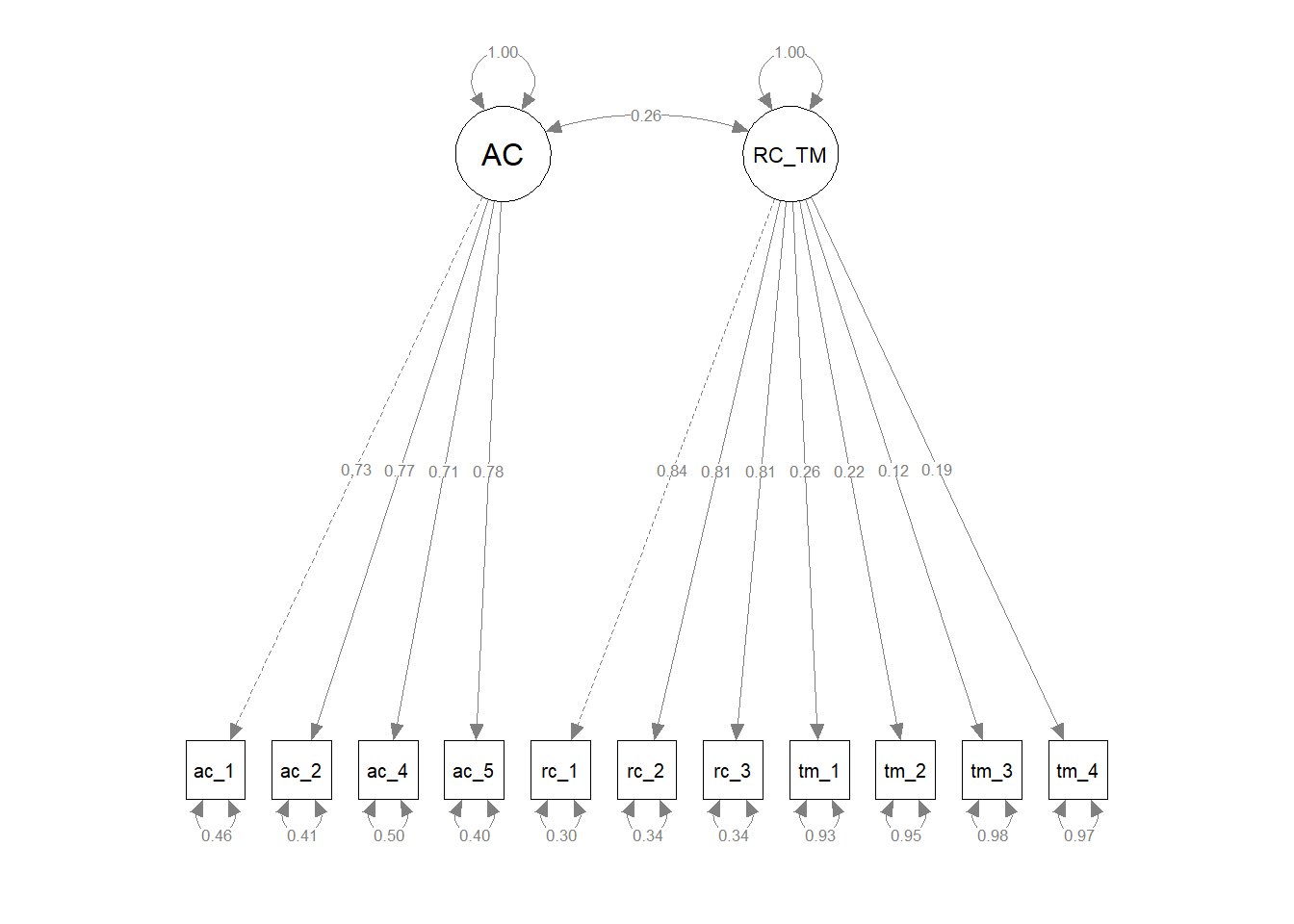

Below, I’ve expanded upon the previous model comparison table by adding in the model fit information for the second version of the two-factor model.

Model	\(\chi^{2}\)	df	p	CFI	TLI	RMSEA	SRMR
3-Factor Model	113.309	41	< .001	.976	.968	.052	.032
2a-Factor Model	994.577	43	< .001	.689	.602	.184	.137
2b-Factor Model	1114.237	43	< .001	.650	.552	.195	.173

As you can see above, the second version (version b) of the two-factor model also fits the data notably worse than the three-factor model, which suggests that the three-factor model is still probably a better representation of the measurement structure.

As before, we’ll also estimate the chi-square (\(\chi^{2}\)) difference test, except this time we’ll compare the three-factor model (cfa_fit_3) to the second version of the two-factor model (cfa_fit_2b).

# Nested model comparison
anova(cfa_fit_3, cfa_fit_2b)

## 
## Chi-Squared Difference Test
## 
##            Df   AIC   BIC   Chisq Chisq diff  RMSEA Df diff            Pr(>Chisq)    
## cfa_fit_3  41 22069 22182  113.31                                                    
## cfa_fit_2b 43 23066 23169 1114.24     1000.9 0.8739       2 < 0.00000000000000022 ***
## ---
## Signif. codes:  0 '***' 0.001 '**' 0.01 '*' 0.05 '.' 0.1 ' ' 1

The chi-square difference test indicates that the second version of the two-factor model fits the data statistically significantly worse than the original three-factor model (\(\Delta \chi^{2}\) = 1000.90, \(\Delta df\) = 2, \(p\) < .001). This corroborates what we saw with the direct comparison of model fit indices above.

57.2.6.3 Two-Factor Model (Version c)

We’ll now evaluate a third version of a two-factor model (version c). In this version, we’ll collapse latent factors AC and TM into a single latent factor and load their respective items on the single factor labeled AC_TM. We’ll specify the RC latent factor such that only the corresponding role clarity items load on it.

# Specify two-factor CFA model & assign to object (version c)
cfa_mod_2c <- "
AC_TM =~ ac_1 + ac_2 + ac_4 + ac_5 + tm_1 + tm_2 + tm_3 + tm_4
RC =~ rc_1 + rc_2 + rc_3 
"

# Estimate three-factor CFA model & assign to fitted model object
cfa_fit_2c <- cfa(cfa_mod_2c, # name of specified model object
                  data=df)    # name of data frame object

# Print summary of model results
summary(cfa_fit_2c,          # name of fitted model object
        fit.measures=TRUE,   # request model fit indices
        standardized=TRUE)   # request standardized estimates

## lavaan 0.6.15 ended normally after 32 iterations
## 
##   Estimator                                         ML
##   Optimization method                           NLMINB
##   Number of model parameters                        23
## 
##   Number of observations                           654
## 
## Model Test User Model:
##                                                       
##   Test statistic                              1059.402
##   Degrees of freedom                                43
##   P-value (Chi-square)                           0.000
## 
## Model Test Baseline Model:
## 
##   Test statistic                              3111.443
##   Degrees of freedom                                55
##   P-value                                        0.000
## 
## User Model versus Baseline Model:
## 
##   Comparative Fit Index (CFI)                    0.667
##   Tucker-Lewis Index (TLI)                       0.575
## 
## Loglikelihood and Information Criteria:
## 
##   Loglikelihood user model (H0)             -11482.743
##   Loglikelihood unrestricted model (H1)     -10953.042
##                                                       
##   Akaike (AIC)                               23011.486
##   Bayesian (BIC)                             23114.597
##   Sample-size adjusted Bayesian (SABIC)      23041.572
## 
## Root Mean Square Error of Approximation:
## 
##   RMSEA                                          0.190
##   90 Percent confidence interval - lower         0.180
##   90 Percent confidence interval - upper         0.200
##   P-value H_0: RMSEA <= 0.050                    0.000
##   P-value H_0: RMSEA >= 0.080                    1.000
## 
## Standardized Root Mean Square Residual:
## 
##   SRMR                                           0.157
## 
## Parameter Estimates:
## 
##   Standard errors                             Standard
##   Information                                 Expected
##   Information saturated (h1) model          Structured
## 
## Latent Variables:
##                    Estimate  Std.Err  z-value  P(>|z|)   Std.lv  Std.all
##   AC_TM =~                                                              
##     ac_1              1.000                               0.940    0.730
##     ac_2              1.035    0.060   17.176    0.000    0.973    0.761
##     ac_4              0.922    0.058   15.797    0.000    0.866    0.690
##     ac_5              1.070    0.063   16.858    0.000    1.006    0.743
##     tm_1              0.548    0.070    7.847    0.000    0.515    0.337
##     tm_2              0.450    0.067    6.684    0.000    0.423    0.286
##     tm_3              0.404    0.067    6.035    0.000    0.380    0.258
##     tm_4              0.475    0.067    7.073    0.000    0.447    0.303
##   RC =~                                                                 
##     rc_1              1.000                               1.157    0.847
##     rc_2              0.970    0.044   22.106    0.000    1.121    0.814
##     rc_3              0.924    0.042   22.204    0.000    1.069    0.819
## 
## Covariances:
##                    Estimate  Std.Err  z-value  P(>|z|)   Std.lv  Std.all
##   AC_TM ~~                                                              
##     RC                0.287    0.053    5.436    0.000    0.264    0.264
## 
## Variances:
##                    Estimate  Std.Err  z-value  P(>|z|)   Std.lv  Std.all
##    .ac_1              0.774    0.056   13.906    0.000    0.774    0.467
##    .ac_2              0.687    0.053   13.030    0.000    0.687    0.421
##    .ac_4              0.827    0.056   14.784    0.000    0.827    0.524
##    .ac_5              0.820    0.060   13.559    0.000    0.820    0.448
##    .tm_1              2.080    0.118   17.630    0.000    2.080    0.887
##    .tm_2              2.006    0.113   17.767    0.000    2.006    0.918
##    .tm_3              2.017    0.113   17.830    0.000    2.017    0.933
##    .tm_4              1.973    0.111   17.724    0.000    1.973    0.908
##    .rc_1              0.529    0.051   10.420    0.000    0.529    0.283
##    .rc_2              0.642    0.053   12.153    0.000    0.642    0.338
##    .rc_3              0.562    0.047   11.911    0.000    0.562    0.330
##     AC_TM             0.883    0.088    9.981    0.000    1.000    1.000
##     RC                1.338    0.107   12.463    0.000    1.000    1.000

# Visualize the measurement model
semPaths(cfa_fit_2c,      # name of fitted model object 
         what="std",      # display standardized parameter estimates
         weighted=FALSE,  # do not weight plot features
         nCharNodes=0)    # do not abbreviate names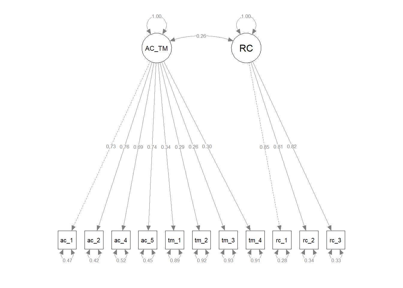

Below, I’ve expanded upon the previous model comparison table by adding in the model fit information for the third version of the two-factor model.

Model	\(\chi^{2}\)	df	p	CFI	TLI	RMSEA	SRMR
3-Factor Model	113.309	41	< .001	.976	.968	.052	.032
2a-Factor Model	994.577	43	< .001	.689	.602	.184	.137
2b-Factor Model	1114.237	43	< .001	.650	.552	.195	.173
2c-Factor Model	1059.402	43	< .001	.667	.575	.190	.157

As you can see above, the third version (version c) of the two-factor model also fits the data notably worse than the three-factor model, which suggests that the three-factor model is still probably a better representation of the measurement structure.

As before, we’ll also estimate the chi-square (\(\chi^{2}\)) difference test, except this time we’ll compare the three-factor model (cfa_fit_3) to the third version of the two-factor model (cfa_fit_2c).

# Nested model comparison
anova(cfa_fit_3, cfa_fit_2c)

## 
## Chi-Squared Difference Test
## 
##            Df   AIC   BIC   Chisq Chisq diff   RMSEA Df diff            Pr(>Chisq)    
## cfa_fit_3  41 22069 22182  113.31                                                     
## cfa_fit_2c 43 23012 23115 1059.40     946.09 0.84958       2 < 0.00000000000000022 ***
## ---
## Signif. codes:  0 '***' 0.001 '**' 0.01 '*' 0.05 '.' 0.1 ' ' 1

The chi-square difference test indicates that the third version of the two-factor model fits the data statistically significantly worse than the original three-factor model (\(\Delta \chi^{2}\) = 946.09, \(\Delta df\) = 2, \(p\) < .001). This corroborates what we saw with the direct comparison of model fit indices above.

57.2.6.4 One-Factor Model

We’ll now evaluate a one-factor model. In this version, we’ll collapse all three latent factors (AC, RC, and TM) into a single latent factor and load their respective items on the single factor labeled AC_RC_TM.

# Specify one-factor CFA model & assign to object 
cfa_mod_1 <- "
AC_RC_TM =~ ac_1 + ac_2 + ac_4 + ac_5 + 
rc_1 + rc_2 + rc_3 +
tm_1 + tm_2 + tm_3 + tm_4
"

# Estimate three-factor CFA model & assign to fitted model object
cfa_fit_1 <- cfa(cfa_mod_1, # name of specified model object
                 data=df)    # name of data frame object

# Print summary of model results
summary(cfa_fit_1,           # name of fitted model object
        fit.measures=TRUE,   # request model fit indices
        standardized=TRUE)   # request standardized estimates

## lavaan 0.6.15 ended normally after 29 iterations
## 
##   Estimator                                         ML
##   Optimization method                           NLMINB
##   Number of model parameters                        22
## 
##   Number of observations                           654
## 
## Model Test User Model:
##                                                       
##   Test statistic                              1921.400
##   Degrees of freedom                                44
##   P-value (Chi-square)                           0.000
## 
## Model Test Baseline Model:
## 
##   Test statistic                              3111.443
##   Degrees of freedom                                55
##   P-value                                        0.000
## 
## User Model versus Baseline Model:
## 
##   Comparative Fit Index (CFI)                    0.386
##   Tucker-Lewis Index (TLI)                       0.232
## 
## Loglikelihood and Information Criteria:
## 
##   Loglikelihood user model (H0)             -11913.742
##   Loglikelihood unrestricted model (H1)     -10953.042
##                                                       
##   Akaike (AIC)                               23871.483
##   Bayesian (BIC)                             23970.112
##   Sample-size adjusted Bayesian (SABIC)      23900.262
## 
## Root Mean Square Error of Approximation:
## 
##   RMSEA                                          0.255
##   90 Percent confidence interval - lower         0.246
##   90 Percent confidence interval - upper         0.265
##   P-value H_0: RMSEA <= 0.050                    0.000
##   P-value H_0: RMSEA >= 0.080                    1.000
## 
## Standardized Root Mean Square Residual:
## 
##   SRMR                                           0.200
## 
## Parameter Estimates:
## 
##   Standard errors                             Standard
##   Information                                 Expected
##   Information saturated (h1) model          Structured
## 
## Latent Variables:
##                    Estimate  Std.Err  z-value  P(>|z|)   Std.lv  Std.all
##   AC_RC_TM =~                                                           
##     ac_1              1.000                               0.911    0.708
##     ac_2              1.053    0.064   16.450    0.000    0.959    0.751
##     ac_4              0.931    0.062   15.080    0.000    0.848    0.675
##     ac_5              1.076    0.067   16.006    0.000    0.981    0.725
##     rc_1              0.466    0.065    7.197    0.000    0.424    0.311
##     rc_2              0.482    0.065    7.384    0.000    0.440    0.319
##     rc_3              0.431    0.062    6.973    0.000    0.393    0.301
##     tm_1              0.612    0.073    8.407    0.000    0.558    0.364
##     tm_2              0.505    0.070    7.211    0.000    0.460    0.311
##     tm_3              0.441    0.070    6.339    0.000    0.402    0.273
##     tm_4              0.524    0.070    7.498    0.000    0.478    0.324
## 
## Variances:
##                    Estimate  Std.Err  z-value  P(>|z|)   Std.lv  Std.all
##    .ac_1              0.827    0.058   14.366    0.000    0.827    0.499
##    .ac_2              0.713    0.054   13.295    0.000    0.713    0.436
##    .ac_4              0.858    0.057   14.992    0.000    0.858    0.544
##    .ac_5              0.870    0.062   13.985    0.000    0.870    0.475
##    .rc_1              1.686    0.095   17.697    0.000    1.686    0.903
##    .rc_2              1.706    0.097   17.674    0.000    1.706    0.898
##    .rc_3              1.550    0.087   17.723    0.000    1.550    0.909
##    .tm_1              2.035    0.116   17.530    0.000    2.035    0.867
##    .tm_2              1.973    0.112   17.695    0.000    1.973    0.903
##    .tm_3              2.000    0.112   17.792    0.000    2.000    0.925
##    .tm_4              1.945    0.110   17.659    0.000    1.945    0.895
##     AC_RC_TM          0.830    0.087    9.571    0.000    1.000    1.000

# Visualize the measurement model
semPaths(cfa_fit_1,       # name of fitted model object 
         what="std",      # display standardized parameter estimates
         weighted=FALSE,  # do not weight plot features
         nCharNodes=0)    # do not abbreviate names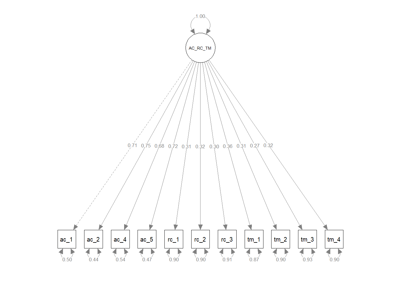

Below, I’ve expanded upon the previous model comparison table by adding in the model fit information for the one-factor model.

Model	\(\chi^{2}\)	df	p	CFI	TLI	RMSEA	SRMR
3-Factor Model	113.309	41	< .001	.976	.968	.052	.032
2a-Factor Model	994.577	43	< .001	.689	.602	.184	.137
2b-Factor Model	1114.237	43	< .001	.650	.552	.195	.173
2c-Factor Model	1059.402	43	< .001	.667	.575	.190	.157
1-Factor Model	1921.400	44	< .001	.386	.232	.255	.200

As you can see above, the one-factor model also fits the data notably worse than the three-factor model, which suggests that the three-factor model remains the best representation of the measurement structure out of the models tested. This gives us more confidence that the three-factor model in which we distinguish between the constructs of feelings of acceptance, role clarity, and task mastery is a solid measurement structure, even though it is the most complex model (in terms of the number of freely estimated parameters) that we evaluated and compared.

As before, though, we’ll also estimate the chi-square (\(\chi^{2}\)) difference test, except this time we’ll compare the three-factor model (cfa_fit_3) to the one-factor model (cfa_fit_1).

# Nested model comparison
anova(cfa_fit_3, cfa_fit_1)

## 
## Chi-Squared Difference Test
## 
##           Df   AIC   BIC   Chisq Chisq diff   RMSEA Df diff            Pr(>Chisq)    
## cfa_fit_3 41 22069 22182  113.31                                                     
## cfa_fit_1 44 23872 23970 1921.40     1808.1 0.95918       3 < 0.00000000000000022 ***
## ---
## Signif. codes:  0 '***' 0.001 '**' 0.01 '*' 0.05 '.' 0.1 ' ' 1

The chi-square difference test indicates that the one-factor model fits the data statistically significantly worse than the original three-factor model (\(\Delta \chi^{2}\) = 1808.10, \(\Delta df\) = 3, \(p\) < .001). This corroborates what we saw with the direct comparison of model fit indices above.

Results write-up for nested model comparisons. As part of a new-employee onboarding survey administered 1-month after employees’ respective start dates, we assessed new employees using three multi-item measures designed to measure feelings of acceptance, role clarity, and task mastery. Guided by theory, we began by estimating a three-factor confirmatory factor analysis (CFA) model, where each construct had an associated latent factor and where each set of items loaded on its corresponding latent factor. We used the the maximum likelihood (ML) estimator to estimate the model, and missing data were not a concern. The three-factor model showed acceptable fit to the data (\(\chi^{2}\) = 113.309, df = 41, p < .001; CFI = .976; TLI = .968; RMSEA = .052; SRMR = .032). We subsequently compared the three-factor model to more parsimonious two- and one-factor models to determine whether any of the alternative models fit the data the data approximately the same with a simpler measurement structure. For the first two-factor model, we collapsed the feelings of acceptance and role clarity latent factors into a single factor and both corresponding measures’ items loaded onto the single latent factor; the task mastery latent factor and its associated items remained a separate latent factor. The first two-factor model showed unacceptable fit to the data (\(\chi^{2}\) = 994.577, df = 43, p < .001; CFI = .689; TLI = .602; RMSEA = .184; SRMR = .137), and a chi-square difference test indicated that this two-factor model fit the data significantly worse than the three-factor model (\(\Delta \chi^{2}\) = 881.27, \(\Delta df\) = 2, p < .001). For the second two-factor model, we collapsed the role clarity and task mastery latent factors into a single factor and both corresponding measures’ items loaded onto the single latent factor; the feelings of acceptance latent factor and its associated items remained a separate latent factor. The first two-factor model showed unacceptable fit to the data (\(\chi^{2}\) = 1114.237, df = 43, p < .001; CFI = .650; TLI = .552; RMSEA = .195; SRMR = .173), and a chi-square difference test indicated that this two-factor model fit the data significantly worse than the three-factor model (\(\Delta \chi^{2}\) = 1000.90, \(\Delta df\) = 2, p < .001). For the third two-factor model, we collapsed the feelings of acceptance and task mastery latent factors into a single factor and both corresponding measures’ items loaded onto the single latent factor; the role clarity latent factor and its associated items remained a separate latent factor. The first two-factor model showed unacceptable fit to the data (\(\chi^{2}\) = 1059.402, df = 43, p < .001; CFI = .667; TLI = .575; RMSEA = .190; SRMR = .157), and a chi-square difference test indicated that this two-factor model fit the data significantly worse than the three-factor model (\(\Delta \chi^{2}\) = 946.09, \(\Delta df\) = 2, p < .001). For the one-factor model, we collapsed the feelings of acceptance, role clarity, and task mastery latent factors into a single factor and all three corresponding measures’ items loaded onto the single latent factor. The first two-factor model showed unacceptable fit to the data (\(\chi^{2}\) = 1921.400, df = 43, p < .001; CFI = .386; TLI = .232; RMSEA = .255; SRMR = .200), and a chi-square difference test indicated that this two-factor model fit the data significantly worse than the three-factor model (\(\Delta \chi^{2}\) = 1808.10, \(\Delta df\) = 3, p < .001). In conclusion, we opted to retain the three-factor model because it fit the data significantly better than the alternative models, even though the three-factor model is more complex and thus sacrifices some degree of parsimony.

57.2.6.5 Create a Matrix Comparing Model Fit Indices

If our goals are to create a matrix containing only those model fit indices that we covered in this chapter and to add in the chi-square difference tests, we can do the following, which incorporates the inspect function from the lavaan package and the cbind, rbind, and t functions from base R.

# Create object containing selected fit indices
select_fit_indices <- c("chisq","df","pvalue","cfi","tli","rmsea","srmr")

# Create matrix comparing model fit indices
compare_mods <- cbind(
  inspect(cfa_fit_3, "fit.indices")[select_fit_indices],
  inspect(cfa_fit_2a, "fit.indices")[select_fit_indices], 
  inspect(cfa_fit_2b, "fit.indices")[select_fit_indices], 
  inspect(cfa_fit_2c, "fit.indices")[select_fit_indices], 
  inspect(cfa_fit_1, "fit.indices")[select_fit_indices]
  )

# Add more informative model names to matrix columns
colnames(compare_mods) <- c("3 Factor Model", 
                            "2a Factor Model",
                            "2b Factor Model",
                            "2c Factor Model",
                            "1 Factor Model")

# Create vector of chi-square difference tests (nested model comparisons)
`chisq diff (p-value)` <- c(NA,
                            anova(cfa_fit_3, cfa_fit_2a)$`Pr(>Chisq)`[2],
                            anova(cfa_fit_3, cfa_fit_2b)$`Pr(>Chisq)`[2],
                            anova(cfa_fit_3, cfa_fit_2c)$`Pr(>Chisq)`[2],
                            anova(cfa_fit_3, cfa_fit_1)$`Pr(>Chisq)`[2])

# Add chi-square difference tests to matrix object
compare_mods <- rbind(compare_mods, `chisq diff (p-value)`)

# Round object values to 3 places after decimal
compare_mods <- round(compare_mods, 3)

# Rotate matrix
compare_mods <- t(compare_mods)

# Print object
print(compare_mods)

##                    chisq df pvalue   cfi   tli rmsea  srmr chisq diff (p-value)
## 3 Factor Model   113.309 41      0 0.976 0.968 0.052 0.032                   NA
## 2a Factor Model  994.577 43      0 0.689 0.602 0.184 0.137                    0
## 2b Factor Model 1114.237 43      0 0.650 0.552 0.195 0.173                    0
## 2c Factor Model 1059.402 43      0 0.667 0.575 0.190 0.157                    0
## 1 Factor Model  1921.400 44      0 0.386 0.232 0.255 0.200                    0

57.2.7 Estimate Second-Order Model

In some instances, we have theoretical justification to specify and estimate a second-order model. A second-order is as CFA model in which latent factors serves as indicators for one or more superordinate latent factors. Let’s suppose that we have theoretical justification to specify a second-order model, where the feelings of acceptance (AC), role clarity (RC), and task mastery (TM) latent factors serve as indicators for a higher-order adjustment latent factor (ADJ). That is, conceptually, an individual’s level of adjustment is indicated by their feelings of acceptance, role clarity, and task mastery. Such a model might prove advantageous if a later goal is to estimate structural regression paths with other criteria, such that just the associations with the second-order adjustment latent factor (ADJ) are of interest.

Specifying a second-order factor is relatively straightforward. To our updated three-factor model, where the ac_3 item was removed, we will specify a second-order factor called ADJ on which the first-order AC, RC, and TM latent factors load: ADJ =~ AC + RC + TM.

# Specify second-order CFA model & assign to object
cfa_mod_2ord <- "
AC =~ ac_1 + ac_2 + ac_4 + ac_5
RC =~ rc_1 + rc_2 + rc_3
TM =~ tm_1 + tm_2 + tm_3 + tm_4
ADJ =~ AC + RC + TM
"

# Estimate second-order CFA model & assign to fitted model object
cfa_fit_2ord <- cfa(cfa_mod_2ord,  # name of specified model object
                    data=df)       # name of data frame object

# Print summary of model results
summary(cfa_fit_2ord,        # name of fitted model object
        fit.measures=TRUE,   # request model fit indices
        standardized=TRUE)   # request standardized estimates

## lavaan 0.6.15 ended normally after 40 iterations
## 
##   Estimator                                         ML
##   Optimization method                           NLMINB
##   Number of model parameters                        25
## 
##   Number of observations                           654
## 
## Model Test User Model:
##                                                       
##   Test statistic                               113.309
##   Degrees of freedom                                41
##   P-value (Chi-square)                           0.000
## 
## Model Test Baseline Model:
## 
##   Test statistic                              3111.443
##   Degrees of freedom                                55
##   P-value                                        0.000
## 
## User Model versus Baseline Model:
## 
##   Comparative Fit Index (CFI)                    0.976
##   Tucker-Lewis Index (TLI)                       0.968
## 
## Loglikelihood and Information Criteria:
## 
##   Loglikelihood user model (H0)             -11009.696
##   Loglikelihood unrestricted model (H1)     -10953.042
##                                                       
##   Akaike (AIC)                               22069.392
##   Bayesian (BIC)                             22181.470
##   Sample-size adjusted Bayesian (SABIC)      22102.095
## 
## Root Mean Square Error of Approximation:
## 
##   RMSEA                                          0.052
##   90 Percent confidence interval - lower         0.041
##   90 Percent confidence interval - upper         0.063
##   P-value H_0: RMSEA <= 0.050                    0.372
##   P-value H_0: RMSEA >= 0.080                    0.000
## 
## Standardized Root Mean Square Residual:
## 
##   SRMR                                           0.032
## 
## Parameter Estimates:
## 
##   Standard errors                             Standard
##   Information                                 Expected
##   Information saturated (h1) model          Structured
## 
## Latent Variables:
##                    Estimate  Std.Err  z-value  P(>|z|)   Std.lv  Std.all
##   AC =~                                                                 
##     ac_1              1.000                               0.946    0.735
##     ac_2              1.041    0.059   17.496    0.000    0.984    0.770
##     ac_4              0.940    0.058   16.301    0.000    0.889    0.708
##     ac_5              1.105    0.063   17.530    0.000    1.045    0.772
##   RC =~                                                                 
##     rc_1              1.000                               1.156    0.846
##     rc_2              0.970    0.044   22.118    0.000    1.122    0.814
##     rc_3              0.925    0.042   22.213    0.000    1.069    0.819
##   TM =~                                                                 
##     tm_1              1.000                               1.159    0.757
##     tm_2              0.951    0.053   17.801    0.000    1.103    0.746
##     tm_3              0.964    0.053   18.103    0.000    1.117    0.760
##     tm_4              0.988    0.054   18.445    0.000    1.145    0.777
##   ADJ =~                                                                
##     AC                1.000                               0.573    0.573
##     RC                0.901    0.259    3.472    0.001    0.422    0.422
##     TM                0.912    0.264    3.461    0.001    0.426    0.426
## 
## Variances:
##                    Estimate  Std.Err  z-value  P(>|z|)   Std.lv  Std.all
##    .ac_1              0.763    0.055   13.832    0.000    0.763    0.460
##    .ac_2              0.665    0.052   12.770    0.000    0.665    0.407
##    .ac_4              0.788    0.054   14.466    0.000    0.788    0.499
##    .ac_5              0.740    0.058   12.699    0.000    0.740    0.404
##    .rc_1              0.530    0.051   10.446    0.000    0.530    0.284
##    .rc_2              0.641    0.053   12.152    0.000    0.641    0.338
##    .rc_3              0.562    0.047   11.916    0.000    0.562    0.330
##    .tm_1              1.002    0.074   13.528    0.000    1.002    0.427
##    .tm_2              0.969    0.070   13.830    0.000    0.969    0.444
##    .tm_3              0.913    0.068   13.433    0.000    0.913    0.422
##    .tm_4              0.861    0.067   12.892    0.000    0.861    0.396
##    .AC                0.601    0.108    5.572    0.000    0.672    0.672
##    .RC                1.099    0.115    9.553    0.000    0.822    0.822
##    .TM                1.100    0.129    8.532    0.000    0.819    0.819
##     ADJ               0.293    0.100    2.942    0.003    1.000    1.000

# Estimate average variance extracted (AVE)
AVE(cfa_fit_2ord)

##    AC    RC    TM 
## 0.559 0.683 0.578

# Estimate composite/construct reliability (CR)
compRelSEM(cfa_fit_2ord)

##    AC    RC    TM 
## 0.835 0.866 0.845

# Visualize the measurement model
semPaths(cfa_fit_2ord,       # name of fitted model object 
         what="std",      # display standardized parameter estimates
         weighted=FALSE,  # do not weight plot features
         nCharNodes=0)    # do not abbreviate names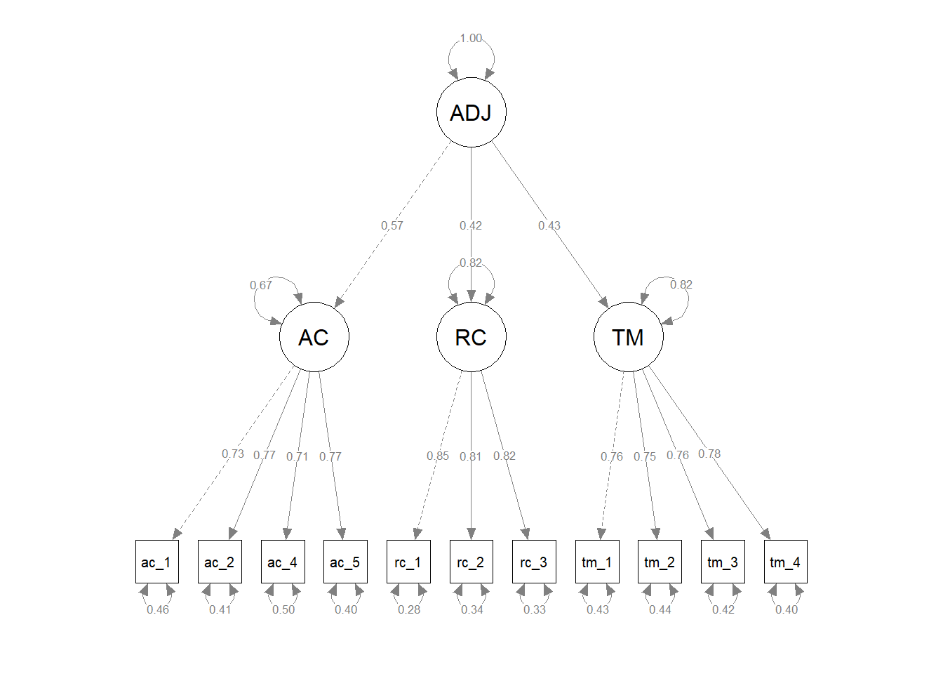

The second-order model fits the data the same as our original first-order three-factor model. A notable difference in the parameter estimates is that instead of covariances between the first-order latent factors (AC, RC, TM), we now see the three latent factors loading onto the new second-order factor (ADJ). We would precede with evaluating and interpreting the model as we did earlier in the chapter with multi-factor models.

57.2.8 Estimating Models with Missing Data

When missing data are present, we must carefully consider how we handle the missing data before or during the estimations of a model. In the chapter on missing data, I provide an overview of relevant concepts, particularly if the data are missing completely at random (MCAR), missing at random (MAR), or missing not at random (MNAR); I suggest reviewing that chapter prior to handling missing data.

As a potential method for addressing missing data, the lavaan model functions, such as the cfa function, allow for full-information maximum likelihood (FIML). Further, the functions allow us to specify specific estimators given the type of data we wish to use for model estimation (e.g., ML, MLR).

To demonstrate how missing data are handled using FIML, we will need to first introduce some missing data into our data. To do so, we will use a multiple imputation package called mice and a function called ampute that “amputates” existing data by creating missing data patterns. For our purposes, we’ll replace 10% (.1) of data frame cells with NA (which is signifies a missing value) such that the missing data are missing completely at random (MCAR).

# Install package
install.packages("mice")

# Access package
library(mice)

# Create a new data frame object
df_missing <- df

# Remove non-numeric variable(s) from data frame object
df_missing$EmployeeID <- NULL

# Set a seed
set.seed(2024)

# Remove 10% of cells so missing data are MCAR
df_missing <- ampute(df_missing, prop=.1, mech="MCAR")

# Extract the new missing data frame object and overwrite existing object
df_missing <- df_missing$amp

Implementing FIML when missing data are present is relatively straightforward. For example, for the updated one-factor CFA model from a previous section, where we removed the ac_3 item, we can apply FIML in the presence of missing data by adding the missing="fiml" argument to the cfa function.

# Specify one-factor CFA model & assign to object
cfa_mod <- "
AC =~ ac_1 + ac_2 + ac_4 + ac_5
"

# Estimate one-factor CFA model & assign to fitted model object
cfa_fit <- cfa(cfa_mod,         # name of specified model object
               data=df_missing, # name of data frame object
               missing="fiml")  # specify FIML
              
# Print summary of model results
summary(cfa_fit,             # name of fitted model object
        fit.measures=TRUE,   # request model fit indices
        standardized=TRUE)   # request standardized estimates

## lavaan 0.6.15 ended normally after 29 iterations
## 
##   Estimator                                         ML
##   Optimization method                           NLMINB
##   Number of model parameters                        12
## 
##   Number of observations                           654
##   Number of missing patterns                         5
## 
## Model Test User Model:
##                                                       
##   Test statistic                                 1.520
##   Degrees of freedom                                 2
##   P-value (Chi-square)                           0.468
## 
## Model Test Baseline Model:
## 
##   Test statistic                               960.360
##   Degrees of freedom                                 6
##   P-value                                        0.000
## 
## User Model versus Baseline Model:
## 
##   Comparative Fit Index (CFI)                    1.000
##   Tucker-Lewis Index (TLI)                       1.002
##                                                       
##   Robust Comparative Fit Index (CFI)             1.000
##   Robust Tucker-Lewis Index (TLI)                1.002
## 
## Loglikelihood and Information Criteria:
## 
##   Loglikelihood user model (H0)              -3878.824
##   Loglikelihood unrestricted model (H1)      -3878.064
##                                                       
##   Akaike (AIC)                                7781.648
##   Bayesian (BIC)                              7835.445
##   Sample-size adjusted Bayesian (SABIC)       7797.345
## 
## Root Mean Square Error of Approximation:
## 
##   RMSEA                                          0.000
##   90 Percent confidence interval - lower         0.000
##   90 Percent confidence interval - upper         0.071
##   P-value H_0: RMSEA <= 0.050                    0.828
##   P-value H_0: RMSEA >= 0.080                    0.027
##                                                       
##   Robust RMSEA                                   0.000
##   90 Percent confidence interval - lower         0.000
##   90 Percent confidence interval - upper         0.072
##   P-value H_0: Robust RMSEA <= 0.050             0.825
##   P-value H_0: Robust RMSEA >= 0.080             0.028
## 
## Standardized Root Mean Square Residual:
## 
##   SRMR                                           0.006
## 
## Parameter Estimates:
## 
##   Standard errors                             Standard
##   Information                                 Observed
##   Observed information based on                Hessian
## 
## Latent Variables:
##                    Estimate  Std.Err  z-value  P(>|z|)   Std.lv  Std.all
##   AC =~                                                                 
##     ac_1              1.000                               0.949    0.737
##     ac_2              1.041    0.059   17.608    0.000    0.987    0.772
##     ac_4              0.941    0.058   16.144    0.000    0.893    0.710
##     ac_5              1.101    0.063   17.454    0.000    1.044    0.772
## 
## Intercepts:
##                    Estimate  Std.Err  z-value  P(>|z|)   Std.lv  Std.all
##    .ac_1              3.900    0.050   77.247    0.000    3.900    3.027
##    .ac_2              3.914    0.050   78.212    0.000    3.914    3.062
##    .ac_4              3.909    0.049   79.345    0.000    3.909    3.107
##    .ac_5              4.269    0.053   80.476    0.000    4.269    3.155
##     AC                0.000                               0.000    0.000
## 
## Variances:
##                    Estimate  Std.Err  z-value  P(>|z|)   Std.lv  Std.all
##    .ac_1              0.759    0.056   13.670    0.000    0.759    0.457
##    .ac_2              0.659    0.053   12.529    0.000    0.659    0.403
##    .ac_4              0.785    0.055   14.313    0.000    0.785    0.496
##    .ac_5              0.740    0.059   12.520    0.000    0.740    0.404
##     AC                0.900    0.089   10.071    0.000    1.000    1.000

The FIML approach uses all observations in which data are missing on one or more endogenous variables in the model. As you can see in the output, all 654 observations were retained for estimating the model.

Now watch what happens when we remove the missing="fiml" argument in the presence of missing data.

# Specify one-factor CFA model & assign to object
cfa_mod <- "
AC =~ ac_1 + ac_2 + ac_4 + ac_5
"

# Estimate one-factor CFA model & assign to fitted model object
cfa_fit <- cfa(cfa_mod,         # name of specified model object
               data=df_missing) # name of data frame object
              
# Print summary of model results
summary(cfa_fit,             # name of fitted model object
        fit.measures=TRUE,   # request model fit indices
        standardized=TRUE)   # request standardized estimates

## lavaan 0.6.15 ended normally after 21 iterations
## 
##   Estimator                                         ML
##   Optimization method                           NLMINB
##   Number of model parameters                         8
## 
##                                                   Used       Total
##   Number of observations                           637         654
## 
## Model Test User Model:
##                                                       
##   Test statistic                                 1.246
##   Degrees of freedom                                 2
##   P-value (Chi-square)                           0.536
## 
## Model Test Baseline Model:
## 
##   Test statistic                               945.071
##   Degrees of freedom                                 6
##   P-value                                        0.000
## 
## User Model versus Baseline Model:
## 
##   Comparative Fit Index (CFI)                    1.000
##   Tucker-Lewis Index (TLI)                       1.002
## 
## Loglikelihood and Information Criteria:
## 
##   Loglikelihood user model (H0)              -3805.421
##   Loglikelihood unrestricted model (H1)      -3804.798
##                                                       
##   Akaike (AIC)                                7626.841
##   Bayesian (BIC)                              7662.496
##   Sample-size adjusted Bayesian (SABIC)       7637.096
## 
## Root Mean Square Error of Approximation:
## 
##   RMSEA                                          0.000
##   90 Percent confidence interval - lower         0.000
##   90 Percent confidence interval - upper         0.068
##   P-value H_0: RMSEA <= 0.050                    0.857
##   P-value H_0: RMSEA >= 0.080                    0.021
## 
## Standardized Root Mean Square Residual:
## 
##   SRMR                                           0.006
## 
## Parameter Estimates:
## 
##   Standard errors                             Standard
##   Information                                 Expected
##   Information saturated (h1) model          Structured
## 
## Latent Variables:
##                    Estimate  Std.Err  z-value  P(>|z|)   Std.lv  Std.all
##   AC =~                                                                 
##     ac_1              1.000                               0.945    0.734
##     ac_2              1.042    0.061   17.221    0.000    0.985    0.770
##     ac_4              0.953    0.059   16.167    0.000    0.901    0.713
##     ac_5              1.114    0.064   17.282    0.000    1.053    0.774
## 
## Variances:
##                    Estimate  Std.Err  z-value  P(>|z|)   Std.lv  Std.all
##    .ac_1              0.766    0.056   13.627    0.000    0.766    0.462
##    .ac_2              0.664    0.053   12.530    0.000    0.664    0.406
##    .ac_4              0.783    0.055   14.115    0.000    0.783    0.491
##    .ac_5              0.740    0.060   12.395    0.000    0.740    0.400
##     AC                0.893    0.090    9.915    0.000    1.000    1.000

As you can see in the output, the cfa function defaults to listwise deletion when we do not specify that FIML be applied. This results in the number of observations dropping from 654 to 637 for model estimation purposes. A reduction in sample size can negatively affect our statistical power to detect associations or effects that truly exist in the underlying population. To learn more about statistical power, please refer to the chapter on power analysis.

Within the cfa function, we can also specify a specific estimator if we choose to override the default. For example, we could specify the MLR (maximum likelihood with robust standard errors) estimator if we had good reason to. To do so, we would add this argument: estimator="MLR". For a list of other available estimators, you can check out the lavaan package website.

# Specify one-factor CFA model & assign to object
cfa_mod <- "
AC =~ ac_1 + ac_2 + ac_3 + ac_4
"

# Estimate one-factor CFA model & assign to fitted model object
cfa_fit <- cfa(cfa_mod,         # name of specified model object
               data=df_missing, # name of data frame object
               estimator="MLR", # specify type of estimator 
               missing="fiml")  # specify FIML
              
# Print summary of model results
summary(cfa_fit,             # name of fitted model object
        fit.measures=TRUE,   # request model fit indices
        standardized=TRUE)   # request standardized estimates

## lavaan 0.6.15 ended normally after 30 iterations
## 
##   Estimator                                         ML
##   Optimization method                           NLMINB
##   Number of model parameters                        12
## 
##   Number of observations                           654
##   Number of missing patterns                         5
## 
## Model Test User Model:
##                                               Standard      Scaled
##   Test Statistic                                 1.383       1.543
##   Degrees of freedom                                 2           2
##   P-value (Chi-square)                           0.501       0.462
##   Scaling correction factor                                  0.896
##     Yuan-Bentler correction (Mplus variant)                       
## 
## Model Test Baseline Model:
## 
##   Test statistic                               566.170     587.012
##   Degrees of freedom                                 6           6
##   P-value                                        0.000       0.000
##   Scaling correction factor                                  0.964
## 
## User Model versus Baseline Model:
## 
##   Comparative Fit Index (CFI)                    1.000       1.000
##   Tucker-Lewis Index (TLI)                       1.003       1.002
##                                                                   
##   Robust Comparative Fit Index (CFI)                         1.000
##   Robust Tucker-Lewis Index (TLI)                            1.002
## 
## Loglikelihood and Information Criteria:
## 
##   Loglikelihood user model (H0)              -4093.056   -4093.056
##   Scaling correction factor                                  0.961
##       for the MLR correction                                      
##   Loglikelihood unrestricted model (H1)      -4092.365   -4092.365
##   Scaling correction factor                                  0.952
##       for the MLR correction                                      
##                                                                   
##   Akaike (AIC)                                8210.113    8210.113
##   Bayesian (BIC)                              8263.910    8263.910
##   Sample-size adjusted Bayesian (SABIC)       8225.810    8225.810
## 
## Root Mean Square Error of Approximation:
## 
##   RMSEA                                          0.000       0.000
##   90 Percent confidence interval - lower         0.000       0.000
##   90 Percent confidence interval - upper         0.070       0.075
##   P-value H_0: RMSEA <= 0.050                    0.845       0.803
##   P-value H_0: RMSEA >= 0.080                    0.023       0.037
##                                                                   
##   Robust RMSEA                                               0.000
##   90 Percent confidence interval - lower                     0.000
##   90 Percent confidence interval - upper                     0.068
##   P-value H_0: Robust RMSEA <= 0.050                         0.846
##   P-value H_0: Robust RMSEA >= 0.080                         0.020
## 
## Standardized Root Mean Square Residual:
## 
##   SRMR                                           0.008       0.008
## 
## Parameter Estimates:
## 
##   Standard errors                             Sandwich
##   Information bread                           Observed
##   Observed information based on                Hessian
## 
## Latent Variables:
##                    Estimate  Std.Err  z-value  P(>|z|)   Std.lv  Std.all
##   AC =~                                                                 
##     ac_1              1.000                               0.941    0.730
##     ac_2              1.079    0.073   14.762    0.000    1.015    0.794
##     ac_3              0.261    0.067    3.874    0.000    0.246    0.177
##     ac_4              0.928    0.063   14.799    0.000    0.873    0.694
## 
## Intercepts:
##                    Estimate  Std.Err  z-value  P(>|z|)   Std.lv  Std.all
##    .ac_1              3.900    0.050   77.278    0.000    3.900    3.028
##    .ac_2              3.914    0.050   78.171    0.000    3.914    3.061
##    .ac_3              3.795    0.055   69.452    0.000    3.795    2.726
##    .ac_4              3.908    0.049   79.276    0.000    3.908    3.104
##     AC                0.000                               0.000    0.000
## 
## Variances:
##                    Estimate  Std.Err  z-value  P(>|z|)   Std.lv  Std.all
##    .ac_1              0.775    0.063   12.380    0.000    0.775    0.467
##    .ac_2              0.604    0.068    8.926    0.000    0.604    0.370
##    .ac_3              1.877    0.096   19.644    0.000    1.877    0.969
##    .ac_4              0.822    0.061   13.373    0.000    0.822    0.519
##     AC                0.885    0.095    9.314    0.000    1.000    1.000

57.2.9 Simulate Dynamic Fit Index Cutoffs

Dynamic fit index cutoffs represent a more recent advance in evaluating model fit. For years, fixed cutoffs for common fit indices have been criticized because the appropriateness of a particular cutoff depends on a number of data- and model-specific factors. For years, the field has referenced cutoffs recommended by influential studies on model fit like Hu and Bentler (1999); however, such recommended cutoffs were based on a single CFA model and thus may not generalize as well as we’d like them to. To address the limitations of general model fit cutoffs, McNeish and Wolf (2023) developed dynamic fit index cutoffs, which are based on a simulation methodology. Further, Wolf and McNeish (2023) developed a package called dynamic to estimate dynamic fit index cutoffs for specific data sets and specific models.

To explore dynamic fit index cutoffs, we need to install and access the dynamic package (if you haven’t already).

# Install package
install.packages("dynamic")

# Access package
library(dynamic)

As an initial step, we need to specify and estimate a CFA model. Let’s start with a one-factor model. Specifically, we’ll use the the same model we specified for the updated over-identified one-factor model earlier in this chapter in which we dropped the ac_3 item.

# Specify one-factor CFA model & assign to object
cfa_mod <- "
AC =~ ac_1 + ac_2 + ac_4 + ac_5
"

# Estimate one-factor CFA model & assign to fitted model object
cfa_fit <- cfa(cfa_mod,      # name of specified model object
               data=df)      # name of data frame object

As the sole parenthetical argument in the cfaOne function from the dynamic package (which is intended for one-factor models), we will enter the name of our fitted model object (cfa_fit). Please note that because this methodology involves Monte Carlo simulations, it will take a minute (or more) to produce the desired output.

# Set seed for reproducible simulation results
set.seed(2024)

# Compute one-factor model dynamic fit index cutoffs
cfaOne(cfa_fit)

## Your DFI cutoffs: 
##                SRMR RMSEA  CFI
## Level 1: 95/5  .016  .078 .993
## Level 1: 90/10   --    --   --
## 
## Empirical fit indices: 
##  Chi-Square  df p-value   SRMR   RMSEA    CFI
##       1.297   2   0.523  0.006       0      1

The output produces the prescribed dynamic fit index cutoffs under the section labeled Your DFI cutoffs. In this output, only a single “level” of cutoffs are produced, specifically Level 1. Had there been additional levels (i.e., Level 2, Level3), they would have corresponded to progressively more relaxed cutoffs indicating worse fitting models; Level 1 corresponds to cutoffs, that if met, correspond to a better fitting model than, say, Level 2 or Level 3. With our model, the dynamic fit index cutoffs for SRMR, RMSEA, and CFI are .016, .078, and .993, respectively, which means that we would love for our actual model fit indices to be less than the first two cutoffs and greater than the last. In the output section labeled Empirical fit indices, we find our actual model fit indices. As you can see, all three of our model fit indices meet the dynamic fit index cutoffs associated with a good-fitting model. Thus, based on these cutoffs, we can conclude that our model fits the data acceptably, which is the same conclusion we arrived at with the traditional cutoffs we applied earlier in the tutorial.

Let’s switch gears and simulate dynamic fit index cutoffs for a multi-factor model. Specifically, we will use our updated three-factor model from a previous section, where the ac_3 item was dropped, as an example.

# Specify three-factor CFA model & assign to object
cfa_mod_3 <- "
AC =~ ac_1 + ac_2 + ac_4 + ac_5
RC =~ rc_1 + rc_2 + rc_3
TM =~ tm_1 + tm_2 + tm_3 + tm_4
"

# Estimate three-factor CFA model & assign to fitted model object
cfa_fit_3 <- cfa(cfa_mod_3,  # name of specified model object
                 data=df)    # name of data frame object

Because we’re dealing with a multi-factor model, we need to switch over to the cfaHB function from the dynamic package. Again, please note that because this involves a Monte Carlo simulation, it will take a minute or two to generate the output.

# Set seed for reproducible simulation results
set.seed(2024)

# Compute three-factor model dynamic fit indices 
cfaHB(cfa_fit_3)

## Your DFI cutoffs: 
##                SRMR RMSEA  CFI Magnitude
## Level 1: 95/5  .082  .105  .92      .528
## Level 1: 90/10   --    --   --          
## Level 2: 95/5  .124  .156 .857      .518
## Level 2: 90/10   --    --   --          
## 
## Empirical fit indices: 
##  Chi-Square  df p-value   SRMR   RMSEA    CFI
##     113.309  41       0  0.032   0.052  0.976

In this example, the cfaHB function generates two levels (Level 1, Level 2) of dynamic fit index cutoffs, where Level 1 corresponds to cutoffs corresponding to better fitting models. Again, note that the actual (empirical) model fit indices for our three-factor model meet the Level 1 cutoffs for SRMR, RMSEA, and CFI, which suggests that our three-factor model fits the data well.

Because dynamic fit index cutoffs are relatively new, we do not yet know whether they will gain broader traction. Still, their use makes conceptual sense, and they may be ushering in a notable shift in how we evaluate model fit.

57.2.10 Summary

In this chapter, we learned how to estimate measurement models using confirmatory factor analysis (CFA). More specifically, we learned how to estimate and interpret one-factor models, multi-factor models, and second-order models, and how to compare the fit of nested models. Further, we learned how to estimate models when missing data are present and how to estimate dynamic fit index cutoffs based on Monte Carlo simulations.

References

Bagozzi, Richard P, and Youjae Yi. 1988. “On the Evaluation of Structural Equation Models.” Journal of the Academy of Marketing Science 16: 74–94.

Bentler, Peter M. 1968. “Alpha-Maximized Factor Analysis (Alphamax): Its Relation to Alpha and Canonical Factor Analysis.” Psychometrika 33 (3): 335–45.

Fornell, Claes, and David F Larcker. 1981. “Evaluating Structural Equation Models with Unobservable Variables and Measurement Errors.” Journal of Marketing Research 18 (1): 39–50.

Hu, Li-tze, and Peter M Bentler. 1999. “Cutoff Criteria for Fit Indexes in Covariance Structure Analysis: Conventional Criteria Versus New Alternatives.” Structural Equation Modeling 6 (1): 1–55.

Kline, Rex B. 2011. Principles and Practice of Structural Equation Modeling (3rd Ed.). New York, New York: The Guilford Press.

McNeish, Daniel, and Melissa G Wolf. 2023. “Dynamic Fit Index Cutoffs for Confirmatory Factor Analysis Models.” Psychological Methods 28 (1): 61–88.

Nye, Christopher D. 2023. “Reviewer Resources: Confirmatory Factor Analysis.” Organizational Research Methods 26 (4): 608–28.

Wickham, Hadley, Jim Hester, and Jennifer Bryan. 2024. Readr: Read Rectangular Text Data. https://CRAN.R-project.org/package=readr.

Wolf, Melissa G, and Daniel McNeish. 2023. “Dynamic: An r Package for Deriving Dynamic Fit Index Cutoffs for Factor Analysis.” Multivariate Behavioral Research 58 (1): 189–94.