Chapter 55 Investigating Processes Using Path Analysis
In this chapter, we will learn how to apply path analysis in order to investigate processes that influence employees’ performance of a particular behavior.
55.1 Conceptual Overview
In its simplest forms, path analysis can represent a single linear regression model (i.e., one outcome, one predictor), but in its more complex, path analysis can represent a system of multiple equations. Path analysis is often useful for testing theoretical or conceptual models with multiple outcome variables and/or outcome variables that also serve as predictor variables (e.g., mediators). Both conventional multiple linear regression modeling and structural equation modeling can be used for path analysis, and in this tutorial we will focus on the latter approach, as it allows for model estimation in a single step and the assessment of overall model fit to the data across the equations specified in the model.
Path analysis can be used to evaluate models with presumed causal chains of variables, and this is why the approach is sometimes called causal modeling. We should be careful with how we use the term causal modeling, however, as showing that a chain of variables are linked to together in a model does not necessarily mean that the variables are causally related.
In this chapter, we will focus on recursive models, which means the direct relations between two variables presumed to be causally related can only be unidirectional. A nonrecursive model allows for bidirectional associations between variables presumed to be causally related and for a predictor variable to be correlated with the residual error of its presumed outcome variable.
55.1.1 Path Diagram
It is customary to depict a path analysis model visually using a path diagram, and as mentioned above, path analysis can be used to test a theoretical or conceptual model of interest. Let’s use the Theory of Planned Behavior (Ajzen 1991). For a simplified version of the theory, please refer to the Figure 1 below.
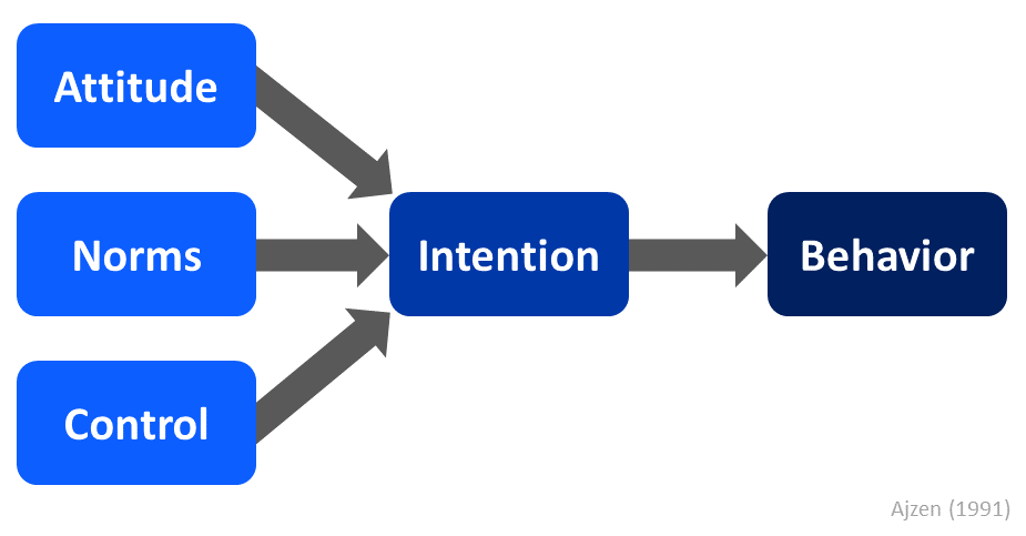
In a simplified form, the Theory of Planned Behavior posits that an intention to perform a particular behavior influences the individual’s decision to enact that behavior, and attitude toward the behavior, perception of norms pertaining to that behavior, and perception of control over performing that behavior influence the individual’s intention to perform the behavior.
We can specify the Theory of Planned Behavior as a path diagram by first drawing the (manifest, observed) variables and the directional (structural) relations (paths) between the variables as implied by the theory, where rectangles represent the variables and directional arrows represent the directional relations between variables, which is depicted in the path diagram below (see Figure 2).
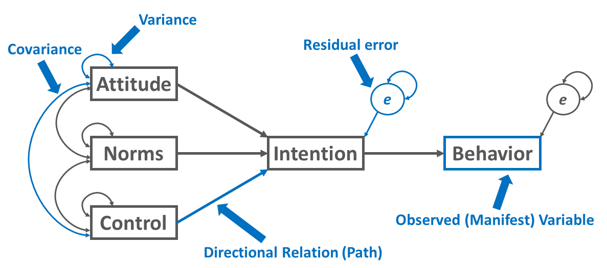
For exogenous variables in the model, on the one hand, we can choose to estimate their variances and the covariances between them; on the other hand, we can choose not to estimate their variances and covariances between them. For our purposes, we’ll practice specifying the variances and covariances between exogenous variables, but note that when missing data are present and full information maximum likelihood is deployed, the decision to estimate the variances of exogenous variables can have additional implications, which go beyond the scope of this tutorial. Exogenous variables serve only as predictor variables in the model, meaning that no other variables in the model to predict them and their causes exist outside of the model. As shown in the figure above, variances are typically represented as curved double-sided arrows, where both arrows point to the same variable. Covariances are also represented as double-sided arrows in which the arrows connect two distinct variables.
(Residual) error terms (which are sometimes called disturbances) are added to endogenous variables, where endogenous variables refer to those variables that are predicted by another variable in the model, meaning that at least one presumed cause is modeled. Note that an endogenous variable may also be specified as the predictor of another endogenous variable, as is the case in our example path diagram representing the Theory of Planned Behavior. In addition, please note that an error term represents variability in an endogenous variable that remains unexplained even after the effects of the specified predictor variables are accounted for. Note, for example, that when we have multiple endogenous variables at the same stage of the model (e.g., first-stage mediators, terminal outcomes), we may choose to allow their error terms to covary.
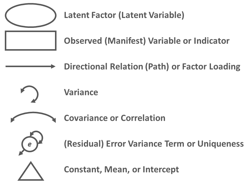
In sum, the conventional symbols used in a path diagram are shown Figure 3 below. With the exception of the manifest variable symbol, all of these symbols represent components of the model that can be estimated statistically using path analysis. These model components that can (and will) be estimated are commonly referred to as parameters or free parameters.
Importantly, please note that in our path diagram because there are no direct relations specified from Attitude to Behavior, Norms to Behavior, and Control to Behavior, which implies that those direct relations are constrained to zero. If we suspected that, in fact, those direct relations are non-zero, then we would draw direction relations (i.e., single-headed arrows) in our path diagram and estimate their values during path analysis.
55.1.2 Model Identification
Model identification has to do with the number of (free) parameters specified in the model relative to the number of unique (non-redundant) sources of information available, and model implication has important implications for assessing model fit and estimating parameter estimates.
Just-identified: In a just-identified model (i.e., saturated model), the number of parameters (e.g., structural relations, variances) is equal to the number of unique (non-redundant) sources of information, which means that the degrees of freedom (df) is equal to zero. In just-identified models, the model parameters can be estimated, but the model fit cannot be assessed in a meaningful way, aside from the R2 value. As a specific applications of path analysis, simple linear and multiple linear regression models are always just-identified.
Over-identified: In an over-identified model, the number of parameters (e.g., structural relations, variances) is less than the number of unique (non-redundant) sources of information, which means that the degrees of freedom (df) is greater than zero. In over-identified models, the model parameters can be estimated, and the model fit can be assessed.
Under-identified: In an under-identified model, the number of parameters (e.g., structural relations, variances) is greater than the number of unique (non-redundant) sources of information, which means that the degrees of freedom (df) is less than zero. In under-identified models, the model parameters and model fit cannot be estimated. Sometimes we might say that such models are called overparameterized because they have more parameters to be estimated than unique (non-redundant) sources of information.
Most (if not all) statistical software packages that allow structural equation modeling – and, by extension, path analysis – to automatically compute the degrees of freedom for a model or provide an error message if the model is under-identified. As such, we don’t need to count the number of sources of unique (non-redundant) sources of information and free parameters by hand. With that said, to understand model identification and its various forms at a deeper level, it is often helpful to practice calculating the degrees freedom by hand when first learning.
The formula for calculating the number of unique (non-redundant) sources of information available for a particular model is as follows:
\(i = \frac{p(p+1)}{2}\)
where \(p\) is the number of manifest (observed) variables to be modeled. This formula calculates the number of possible unique covariances and variances for the variables specified in the model – or in other words, it calculates the lower diagonal of a covariance matrix, including the variances.
In the path diagram we specified above, there are five manifest variables: Attitude, Norms, Control, Intention, and Behavior. Thus, in the following formula, \(p\) is equal to 5, and thus the number of unique (non-redundant) sources of information is 15.
\(i = \frac{5(5+1)}{2} = \frac{30}{2} = 15\)
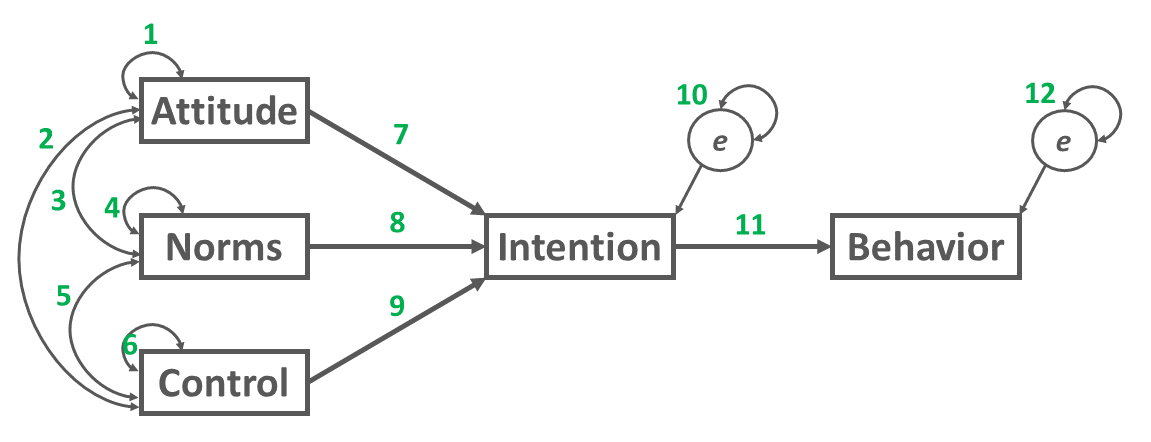
To count the number of free parameters (\(k\)), simply add up the number of the specified direction relations, variances, covariances, and error terms in the path analysis model. As shown in Figure 4 below, our example path analysis model has 12 free parameters.
\(k = 12\)
To calculate the degrees of freedom (df) for the model, subtract the number of free parameters from the number unique (non-redundant) sources of information, which in this example is equal to 3, as shown below. Thus, the degrees of freedom for the model is 3, which means the model is over-identified.
\(df = i - k = 15 - 12 = 3\)
55.1.3 Model Fit
When a model is over-identified (df > 0), the extent to which the specified model fits the data can be assessed using various model fit indices, such as the chi-square test (\(\chi^{2}\)), comparative fit index (CFI), Tucker-Lewis index (TLI), root mean square error of approximation (RMSEA), and standardized root mean square residual (SRMR). For a commonly cited reference on cutoffs for fit indices, please refer to Hu and Bentler (1999).
Chi-square test: The chi-square test can be used to assess whether the model fits the data, where a statistically significant chi-square value (e.g., p < .05) indicates that the model does not fit the data well and a nonsignificant chi-square value (e.g., p > .05) indicates that the model fits the data reasonably well. The null hypothesis for the chi-square test is that the model fits the data perfectly, and thus failing to reject the null model provides some confidence that the model fits the data reasonably close to perfectly. The chi-square test is sensitive to sample size and non-normal variable distributions.
Comparative fit index (CFI): As the name implies, the comparative fit index (CFI) is a type of comparative (or incremental) fit index, which means that the CFI compares the focal model to a baseline model, which is commonly referred to as the null or independence model. The CFI is generally less sensitive to sample size than the chi-square test. A CFI value greater than or equal to .90 generally indicates good model fit to the data.
Tucker-Lewis index (TLI): Like the CFI, the Tucker-Lewis index (TLI) is another type of comparative (or incremental) fit index. The TLI is generally less sensitive to sample size than the chi-square test and tends to work well with smaller sample sizes. A TLI value greater than or equal to .95 generally indicates good model fit to the data, although some might relax that cutoff to .90.
Root mean square error of approximation (RMSEA): The root mean square error of approximation (RMSEA) is an absolute fit index that penalizes model complexity (e.g., models with a larger number of estimated parameters) and thus ends up effectively rewarding more parsimonious models. RMSEA values tend to upwardly biased when the model degrees of freedom are fewer (i.e., when the model is closer to being just-identified). In general, an RMSEA value that is less than or equal to .08 indicates good model fit to the data, although some relax that cutoff to .10.
Standardized root mean square residual (SRMR): Like the RMSEA, the standardized root mean square residual (SRMR) is an example of an absolute fit index. An SRMR value that is less than or equal to .08 generally indicates good fit to the data.
Summary of model fit indices: The conventional cutoffs for the aforementioned model fit indices – like any rule of thumb – should be applied with caution and with good judgment and intention. Further, these indices don’t always agree with one another, which means that we often look across multiple fit indices and come up with our best judgment of whether the model adequately fits the data. Generally, it is not advisable to interpret model parameter estimates unless the model fits the data adequately. Below is a table of the conventional cutoffs for the model fit indices.
| Fit Index | Cutoff for Adequate Fit |
|---|---|
| \(\chi^{2}\) | \(p \ge .05\) |
| CFI | \(\ge .90\) |
| TLI | \(\ge .95\) |
| RMSEA | \(\le .08\) |
| SRMR | \(\le .08\) |
55.1.4 Parameter Estimates
In path analysis, parameter estimates (e.g., direct relations, covariances, variances) can be interpreted like those from a regression model, where the associated p-values or confidence intervals can be used as indicators of statistical significance.
55.1.5 Statistical Assumptions
The statistical assumptions that should be met prior to running and/or interpreting a path analysis model overlap with those associated with multiple linear regression, and thus for a review of those assumptions please see the chapter on incremental validity using multiple linear regression.
55.1.6 Conceptual Video
For a more in-depth review of path analysis, please check out the following conceptual video.
Link to conceptual video: https://youtu.be/UGIVPtFKwc0
55.2 Tutorial
This chapter’s tutorial demonstrates estimate a path analysis model using R.
55.2.1 Video Tutorial
As usual, you have the choice to follow along with the written tutorial in this chapter or to watch the video tutorial below.
Link to video tutorial: https://youtu.be/vMStRfsUTBg
55.2.3 Initial Steps
If you haven’t already, save the file called “PlannedBehavior.csv” into a folder that you will subsequently set as your working directory. Your working directory will likely be different than the one shown below (i.e., "H:/RWorkshop"). As a reminder, you can access all of the data files referenced in this book by downloading them as a compressed (zipped) folder from the my GitHub site: https://github.com/davidcaughlin/R-Tutorial-Data-Files; once you’ve followed the link to GitHub, just click “Code” (or “Download”) followed by “Download ZIP”, which will download all of the data files referenced in this book. For the sake of parsimony, I recommend downloading all of the data files into the same folder on your computer, which will allow you to set that same folder as your working directory for each of the chapters in this book.
Next, using the setwd function, set your working directory to the folder in which you saved the data file for this chapter. Alternatively, you can manually set your working directory folder in your drop-down menus by going to Session > Set Working Directory > Choose Directory…. Be sure to create a new R script file (.R) or update an existing R script file so that you can save your script and annotations. If you need refreshers on how to set your working directory and how to create and save an R script, please refer to Setting a Working Directory and Creating & Saving an R Script.
Next, read in the .csv data file called “PlannedBehavior.csv” using your choice of read function. In this example, I use the read_csv function from the readr package (Wickham, Hester, and Bryan 2024). If you choose to use the read_csv function, be sure that you have installed and accessed the readr package using the install.packages and library functions. Note: You don’t need to install a package every time you wish to access it; in general, I would recommend updating a package installation once ever 1-3 months. For refreshers on installing packages and reading data into R, please refer to Packages and Reading Data into R.
# Install readr package if you haven't already
# [Note: You don't need to install a package every
# time you wish to access it]
install.packages("readr")
# Access readr package
library(readr)
# Read data and name data frame (tibble) object
df <- read_csv("PlannedBehavior.csv")## Rows: 199 Columns: 5
## ── Column specification ────────────────────────────────────────────────────────────────────────────────────────────────────────────
## Delimiter: ","
## dbl (5): attitude, norms, control, intention, behavior
##
## ℹ Use `spec()` to retrieve the full column specification for this data.
## ℹ Specify the column types or set `show_col_types = FALSE` to quiet this message.## [1] "attitude" "norms" "control" "intention" "behavior"## spc_tbl_ [199 × 5] (S3: spec_tbl_df/tbl_df/tbl/data.frame)
## $ attitude : num [1:199] 2.31 4.66 3.85 4.24 2.91 2.99 3.96 3.01 4.77 3.67 ...
## $ norms : num [1:199] 2.31 4.01 3.56 2.25 3.31 2.51 4.65 2.98 3.09 3.63 ...
## $ control : num [1:199] 2.03 3.63 4.2 2.84 2.4 2.95 3.77 1.9 3.83 5 ...
## $ intention: num [1:199] 2.5 3.99 4.35 1.51 1.45 2.59 4.08 2.58 4.87 3.09 ...
## $ behavior : num [1:199] 2.62 3.64 3.83 2.25 2 2.2 4.41 4.15 4.35 3.95 ...
## - attr(*, "spec")=
## .. cols(
## .. attitude = col_double(),
## .. norms = col_double(),
## .. control = col_double(),
## .. intention = col_double(),
## .. behavior = col_double()
## .. )
## - attr(*, "problems")=<externalptr>## # A tibble: 6 × 5
## attitude norms control intention behavior
## <dbl> <dbl> <dbl> <dbl> <dbl>
## 1 2.31 2.31 2.03 2.5 2.62
## 2 4.66 4.01 3.63 3.99 3.64
## 3 3.85 3.56 4.2 4.35 3.83
## 4 4.24 2.25 2.84 1.51 2.25
## 5 2.91 3.31 2.4 1.45 2
## 6 2.99 2.51 2.95 2.59 2.2## [1] 199There are 5 variables and 199 cases (i.e., employees) in the df data frame: attitude, norms, control, intention, and behavior. Per the output of the str (structure) function above, all of the variables are of type numeric (continuous: interval/ratio). All of the variables are self-reports from a survey, where respondents rated their level of agreement (1 = strongly disagree, 5 = strongly agree) for the items associated with the attitude, norms, control, and intention scales, and where respondents rated the frequency with which they enact the behavior associated with the behavior variable (1 = never, 5 = all of the time). The attitude variable reflects an employee’s attitude toward the behavior in question. The norms variable reflects an employee’s perception of norms pertaining to the enactment of the behavior. The control variable reflects an employee’s feeling of control over being able to perform the behavior. The intention variable reflects an employee’s intention to enact the behavior. The behavior variable reflects an employee’s perception of the frequency with which they actually engage in the behavior.
55.2.4 Specifying & Estimating Path Analysis Models
We will use functions from the lavaan package (Rosseel 2012) to specify and estimate our path analysis model. The lavaan package also allows structural equation modeling with latent variables, but we won’t cover that in this tutorial. If you haven’t already install and access the lavaan package using the install.packages and library functions, respectively. For background information on the lavaan package, check out the package website.
55.2.4.1 Estimating a Multiple Linear Regression Model Using Path Analysis
Let’s begin by demonstrating how a multiple linear regression model can be estimated using lavaan and it’s functions. Specifically, let’s focus on the first part of our Theory of Planned Behavior model, where attitude, norms, and control are proposed as predictors intention.
- Using the
<-operator, name the specified model object something of your choosing (specmod). To the right of the<-operator, enter quotation marks (" "). Within the quotation marks, specify the model, which in this case is a multiple linear regression equation:
- Regress the outcome variable (
intention) onto the predictor variables (attitude,norms,control). Just like we would with other regression functions in R, we use the tilde (~) to separate our outcome variable from our predictor variable, where the outcome variable goes to the left of the tilde, and the predictor variables go to the right, resulting in the following equation (and specified directional paths/relations):intention ~ attitude + norms + control. - To estimate the model intercept associated with our outcome variable (
intention), we need to explicitly specify the intercept of ofintention, as thesemfunction will not provide these by default with these model specifications. To do so, specify the outcome variable followed by~ 1, which should look like this:intention ~ 1.
- Using the
semfunction fromlavaan, type the name of the specified regression model (specmod) as the first argument anddata=followed by the name of the data from which the variables belong as the second argument. Using the<-operator, name the estimated model object something, and here I name itfitmodfor fitted model. - Using the
summaryfunction from base R, request a summary of the model fit and parameter estimate results.
- As the first argument in the
summaryfunction, type the name of the estimated model function from the previous step (fitmod). - As the second argument, type
fit.measures=TRUEto request the model fit indices as part of the output. - As the third argument, type
rsquare=TRUEto request the unadjusted R2 value for the model.
# Specify path analysis model & assign to object
specmod <- "
# Specify directional paths/relations
intention ~ attitude + norms + control

# Specify model intercept for outcome variable
intention ~ 1
"

# Estimate path analysis model & assign to fitted model object
fitmod <- sem(specmod,  # name of specified model object
              data=df)  # name of data frame object

# Print summary of model results
summary(fitmod,              # name of fitted model object
        fit.measures=TRUE,   # request model fit indices
        rsquare=TRUE)        # request R-squared estimates
## lavaan 0.6.15 ended normally after 15 iterations
##
## Estimator ML
## Optimization method NLMINB
## Number of model parameters 5
##
## Number of observations 199
##
## Model Test User Model:
##
## Test statistic 0.000
## Degrees of freedom 0
##
## Model Test Baseline Model:
##
## Test statistic 91.633
## Degrees of freedom 3
## P-value 0.000
##
## User Model versus Baseline Model:
##
## Comparative Fit Index (CFI) 1.000
## Tucker-Lewis Index (TLI) 1.000
##
## Loglikelihood and Information Criteria:
##
## Loglikelihood user model (H0) -219.244
## Loglikelihood unrestricted model (H1) -219.244
##
## Akaike (AIC) 448.489
## Bayesian (BIC) 464.955
## Sample-size adjusted Bayesian (SABIC) 449.115
##
## Root Mean Square Error of Approximation:
##
## RMSEA 0.000
## 90 Percent confidence interval - lower 0.000
## 90 Percent confidence interval - upper 0.000
## P-value H_0: RMSEA <= 0.050 NA
## P-value H_0: RMSEA >= 0.080 NA
##
## Standardized Root Mean Square Residual:
##
## SRMR 0.000
##
## Parameter Estimates:
##
## Standard errors Standard
## Information Expected
## Information saturated (h1) model Structured
##
## Regressions:
## Estimate Std.Err z-value P(>|z|)
## intention ~
## attitude 0.352 0.058 6.068 0.000
## norms 0.153 0.059 2.577 0.010
## control 0.275 0.058 4.740 0.000
##
## Intercepts:
## Estimate Std.Err z-value P(>|z|)
## .intention 0.586 0.237 2.470 0.014
##
## Variances:
## Estimate Std.Err z-value P(>|z|)
## .intention 0.530 0.053 9.975 0.000
##
## R-Square:
## Estimate
## intention 0.369Towards the top of the output, alongside “Number of observations”, the number 199 appears, which indicates that 199 employees’ data were included in this analysis. Because there were no missing data, all 199 employees were retained in the sample for analysis (instead of being listwise deleted by default). Further below, you will see a zero (0) next to “Degrees of freedom”, which indicates that the model is just-identified. Thus, we will ignore the model fit information and skip down to the “Regressions” section. The path coefficient (i.e., regression coefficient) between attitude and intention is statistically significant and positive (b = .352, p < .001). The path coefficient between norms and intention is statistically significant and positive (b = .153, p = .010). The path coefficient between control and intention is statistically significant and positive (b = .275, p < .001). Beneath the “Intercepts” section, you will find the model intercept value for intention, which is statistically significantly different from zero and positive (b = .589, p = .014). Under the “R-Square” section, we see the unadjusted R2 value for the outcome variable intention, which is equal to .369; that is, collectively, attitude, norms, and control explain 36.9% of the variance in intention.
Using the lm (linear model) function from base R we can verify that our path analysis results using the sem function from lavaan are equivalent to multiple linear regression results from a conventional linear regression function. For a review of the lm function, please refer to the chapter supplement for estimating incremental validity using multiple linear regression.
# Specify & estimate multiple linear regression model
fitmod <- lm(intention ~ attitude + norms + control, data=df)

# Print summary of results
summary(fitmod)
##
## Call:
## lm(formula = intention ~ attitude + norms + control, data = df)
##
## Residuals:
## Min 1Q Median 3Q Max
## -1.80282 -0.52734 -0.06018 0.51228 1.85202
##
## Coefficients:
## Estimate Std. Error t value Pr(>|t|)
## (Intercept) 0.58579 0.23963 2.445 0.0154 *
## attitude 0.35232 0.05866 6.006 0.00000000913 ***
## norms 0.15250 0.05979 2.550 0.0115 *
## control 0.27502 0.05862 4.692 0.00000509027 ***
## ---
## Signif. codes: 0 '***' 0.001 '**' 0.01 '*' 0.05 '.' 0.1 ' ' 1
##
## Residual standard error: 0.7356 on 195 degrees of freedom
## Multiple R-squared: 0.369, Adjusted R-squared: 0.3593
## F-statistic: 38.01 on 3 and 195 DF, p-value: < 0.00000000000000022As you can see, aside from the number of digits reported after the decimal, the lm regression coefficients, model intercept estimate unadjusted R2 value are the same as the corresponding estimates from the model estimated using the sem function. With that said, the standard errors and p-values differ slightly across the two models. The reason being, the sem function uses maximum likelihood (ML) estimation, whereas the lm function uses a type of least squares estimation called ordinary least squares (OLS) estimation. Although a full review and comparison of the differences between ML and OLS estimators is beyond the scope of this chapter, simply put, the OLS estimator and ML estimator carry different assumptions and estimation approaches. Thus, while the substantive results remain the same, there are differences in the standard errors and p-values due to the different estimators applied by the lm and sem functions.
55.2.4.2 Estimating Covariances in a Path Analysis Model
Using path analysis, we can explicitly model the covariances (correlations) between the predictor (exogenous) variables in the model by using the double tilde (~~) operator. As noted above, in a real-life situation, we should carefully consider what it means to add these covariances to exogenous variables, particularly when estimating models in the presence of missing data by using full information maximum likelihood. Briefly, estimating the covariances between exogenous variables assumes the exogenous variables are random variables, with their own freely estimated intercepts and variances. Conversely, by omitting the covariances (i.e., by default, constraining the covariances to zero), the exogenous variables are assumed to be fixed variables, with their intercepts, variances, and covariances constrained to sample estimates. Thus, in this chapter, we are merely specifying the covariances between these exogenous variables to illustrate how to apply double tilde (~~) operator.
Within our model specification quotation marks (" "), we additionally specify the covariances between the exogenous variables (attitude, norms, control). In doing so, we will freely estimate not only the covariances between the exogenous variables, but also their intercepts and variances. To do so, we simply apply the double tilde (~~) operator to capture all three possible covariances between the three exogenous variables. Finally, in this model, we will drop the model intercept (intention ~ 1) that we freely estimated in the path analysis model from the previous section, as that model intercept won’t be of substantive interest for us going forward.
# Specify path analysis model & assign to object
specmod <- "
# Specify directional paths/relations
intention ~ attitude + norms + control

# Specify covariances between exogenous variables
attitude ~~ norms + control
norms ~~ control
"

# Estimate path analysis model & assign to fitted model object
fitmod <- sem(specmod,  # name of specified model object
              data=df)  # name of data frame object

# Print summary of model results
summary(fitmod,              # name of fitted model object
        fit.measures=TRUE,   # request model fit indices
        rsquare=TRUE)        # request R-squared estimates
## lavaan 0.6.15 ended normally after 18 iterations
##
## Estimator ML
## Optimization method NLMINB
## Number of model parameters 10
##
## Number of observations 199
##
## Model Test User Model:
##
## Test statistic 0.000
## Degrees of freedom 0
##
## Model Test Baseline Model:
##
## Test statistic 136.306
## Degrees of freedom 6
## P-value 0.000
##
## User Model versus Baseline Model:
##
## Comparative Fit Index (CFI) 1.000
## Tucker-Lewis Index (TLI) 1.000
##
## Loglikelihood and Information Criteria:
##
## Loglikelihood user model (H0) -1011.828
## Loglikelihood unrestricted model (H1) -1011.828
##
## Akaike (AIC) 2043.656
## Bayesian (BIC) 2076.589
## Sample-size adjusted Bayesian (SABIC) 2044.908
##
## Root Mean Square Error of Approximation:
##
## RMSEA 0.000
## 90 Percent confidence interval - lower 0.000
## 90 Percent confidence interval - upper 0.000
## P-value H_0: RMSEA <= 0.050 NA
## P-value H_0: RMSEA >= 0.080 NA
##
## Standardized Root Mean Square Residual:
##
## SRMR 0.000
##
## Parameter Estimates:
##
## Standard errors Standard
## Information Expected
## Information saturated (h1) model Structured
##
## Regressions:
## Estimate Std.Err z-value P(>|z|)
## intention ~
## attitude 0.352 0.058 6.068 0.000
## norms 0.153 0.059 2.577 0.010
## control 0.275 0.058 4.740 0.000
##
## Covariances:
## Estimate Std.Err z-value P(>|z|)
## attitude ~~
## norms 0.200 0.064 3.128 0.002
## control 0.334 0.070 4.748 0.000
## norms ~~
## control 0.220 0.065 3.411 0.001
##
## Variances:
## Estimate Std.Err z-value P(>|z|)
## .intention 0.530 0.053 9.975 0.000
## attitude 0.928 0.093 9.975 0.000
## norms 0.830 0.083 9.975 0.000
## control 0.939 0.094 9.975 0.000
##
## R-Square:
## Estimate
## intention 0.369First, note that the model degrees of freedom (df) is equal to zero (0), which indicates that this model is just-identified. Second, note that the parameter estimates for the covariances now appear in the output under the section titled “Covariances.” Third, note that the intercepts of the exogenous variables now appear in the section titled “Intercepts.” Fourth, note that the variances of the exogenous variables now appear in the section titled “Variances.”
55.2.4.3 Specifying a More Complex Path Analysis Model
Now it’s time to test a full model of the Theory of Planned Behavior by adding the equation in which intention predicts behavior. We will build on our previous path analysis model script by specifying that intention is a predictor of behavior (i.e., behavior ~ intention). Everything else in our script can remain the same.
# Specify path analysis model & assign to object
specmod <- "
# Specify directional paths/relations
intention ~ attitude + norms + control
behavior ~ intention

# Specify covariances between exogenous variables
attitude ~~ norms + control
norms ~~ control
"

# Estimate path analysis model & assign to fitted model object
fitmod <- sem(specmod,  # name of specified model object
              data=df)  # name of data frame object

# Print summary of model results
summary(fitmod,              # name of fitted model object
        fit.measures=TRUE,   # request model fit indices
        rsquare=TRUE)        # request R-squared estimates
## lavaan 0.6.15 ended normally after 18 iterations
##
## Estimator ML
## Optimization method NLMINB
## Number of model parameters 12
##
## Number of observations 199
##
## Model Test User Model:
##
## Test statistic 2.023
## Degrees of freedom 3
## P-value (Chi-square) 0.568
##
## Model Test Baseline Model:
##
## Test statistic 182.295
## Degrees of freedom 10
## P-value 0.000
##
## User Model versus Baseline Model:
##
## Comparative Fit Index (CFI) 1.000
## Tucker-Lewis Index (TLI) 1.019
##
## Loglikelihood and Information Criteria:
##
## Loglikelihood user model (H0) -1258.517
## Loglikelihood unrestricted model (H1) -1257.506
##
## Akaike (AIC) 2541.035
## Bayesian (BIC) 2580.555
## Sample-size adjusted Bayesian (SABIC) 2542.538
##
## Root Mean Square Error of Approximation:
##
## RMSEA 0.000
## 90 Percent confidence interval - lower 0.000
## 90 Percent confidence interval - upper 0.103
## P-value H_0: RMSEA <= 0.050 0.735
## P-value H_0: RMSEA >= 0.080 0.120
##
## Standardized Root Mean Square Residual:
##
## SRMR 0.019
##
## Parameter Estimates:
##
## Standard errors Standard
## Information Expected
## Information saturated (h1) model Structured
##
## Regressions:
## Estimate Std.Err z-value P(>|z|)
## intention ~
## attitude 0.352 0.058 6.068 0.000
## norms 0.153 0.059 2.577 0.010
## control 0.275 0.058 4.740 0.000
## behavior ~
## intention 0.453 0.065 7.014 0.000
##
## Covariances:
## Estimate Std.Err z-value P(>|z|)
## attitude ~~
## norms 0.200 0.064 3.128 0.002
## control 0.334 0.070 4.748 0.000
## norms ~~
## control 0.220 0.065 3.411 0.001
##
## Variances:
## Estimate Std.Err z-value P(>|z|)
## .intention 0.530 0.053 9.975 0.000
## .behavior 0.699 0.070 9.975 0.000
## attitude 0.928 0.093 9.975 0.000
## norms 0.830 0.083 9.975 0.000
## control 0.939 0.094 9.975 0.000
##
## R-Square:
## Estimate
## intention 0.369
## behavior 0.198Again, we have 199 observations (employees) used in this analysis, but this time, the degrees of freedom is equal to 3, which indicates that our model is over-identified. Because the model is over-identified, we can interpret the model fit indices to assess the how well the model we specified fits the data. First, the chi-square test value appears to the right of the text “Model Fit Test Statistic”, and the associated p-value appears below. The chi-square test is nonsignificant (\(\chi^{2}(df=3)=2.023, p=.568\)), which indicates that the model does not fit significantly worse than a model that fits the data perfectly; thus, we have our first indicator that the model fits the data reasonably well. Second, the comparative fit index (CFI) is 1.000, which is greater than the conventional .90 cutoff, which also indicates that the model fits the data reasonably well. Third, the Tucker-Lewis index (TLI) is 1.019, which is greater than the conventional .95 cutoff, which also indicates that the model fits the data reasonably well. Fourth, the root mean square error of approximation (RMSEA) value of .000 is less than the conventional cutoff of .08, and thus we have further evidence that the model fits the data reasonably well. Fifth, the standardized root mean square residual (SRMR) value of .019 is less than the conventional cutoff of .08, and thus we have further evidence that the model fits the data reasonably well. This is one of the relatively rare occasions in which all of the model fit indices are in agreement with one another, leading us to conclude that the specified model fits the data well. We can now feel comfortable proceeding forward interpreting the parameter estimates.
The path coefficient (i.e., direct relation, presumed causal relation) between attitude and intention is statistically significant and positive (b = .352, p < .001); the path coefficient between norms and intention is also statistically significant and positive (b = .153, p = .010); and the path coefficient between control and intention is also statistically significant and positive (b = .275, p < .001). Further, the path coefficient between intention and behavior is statistically significant and positive (b = .453, p < .001). The covariances and variances are not of substantive interest, so we will ignore them. The unadjusted R2 value for the outcome variable intention is .369, which indicates that, collectively, attitude, norms, and control explain 36.9% of the variance in intention, and the unadjusted R2 value for the outcome variable behavior is .198, which indicates that intention explains 19.8% of the variance in behavior. Overall, the results lends support to the propositions of the Theory of Planned Behavior, at least based on this sample of employees.
In the following chapter, we will learn how to estimate the indirect effects of the predictor variable(s) on the outcome variable(s) via a mediator variable by applying mediation analysis in a path analysis framework.
55.2.5 Obtaining Standardized Parameter Estimates
Just like traditional linear regression models, we sometimes obtain standardized parameter estimates in path analysis models to get a better understanding of the magnitude of the effects. Fortunately, requesting standardized parameter estimates just requires adding the standardized=TRUE to the summary function.
# Specify path analysis model & assign to object
specmod <- "
# Specify directional paths/relations
intention ~ attitude + norms + control
behavior ~ intention

# Specify covariances between exogenous variables
attitude ~~ norms + control
norms ~~ control
"

# Estimate path analysis model & assign to fitted model object
fitmod <- sem(specmod,  # name of specified model object
              data=df)  # name of data frame object

# Print summary of model results
summary(fitmod,              # name of fitted model object
        fit.measures=TRUE,   # request model fit indices
        standardized=TRUE,   # request standardized estimates
        rsquare=TRUE)        # request R-squared estimates
## lavaan 0.6.15 ended normally after 18 iterations
##
## Estimator ML
## Optimization method NLMINB
## Number of model parameters 12
##
## Number of observations 199
##
## Model Test User Model:
##
## Test statistic 2.023
## Degrees of freedom 3
## P-value (Chi-square) 0.568
##
## Model Test Baseline Model:
##
## Test statistic 182.295
## Degrees of freedom 10
## P-value 0.000
##
## User Model versus Baseline Model:
##
## Comparative Fit Index (CFI) 1.000
## Tucker-Lewis Index (TLI) 1.019
##
## Loglikelihood and Information Criteria:
##
## Loglikelihood user model (H0) -1258.517
## Loglikelihood unrestricted model (H1) -1257.506
##
## Akaike (AIC) 2541.035
## Bayesian (BIC) 2580.555
## Sample-size adjusted Bayesian (SABIC) 2542.538
##
## Root Mean Square Error of Approximation:
##
## RMSEA 0.000
## 90 Percent confidence interval - lower 0.000
## 90 Percent confidence interval - upper 0.103
## P-value H_0: RMSEA <= 0.050 0.735
## P-value H_0: RMSEA >= 0.080 0.120
##
## Standardized Root Mean Square Residual:
##
## SRMR 0.019
##
## Parameter Estimates:
##
## Standard errors Standard
## Information Expected
## Information saturated (h1) model Structured
##
## Regressions:
## Estimate Std.Err z-value P(>|z|) Std.lv Std.all
## intention ~
## attitude 0.352 0.058 6.068 0.000 0.352 0.370
## norms 0.153 0.059 2.577 0.010 0.153 0.152
## control 0.275 0.058 4.740 0.000 0.275 0.291
## behavior ~
## intention 0.453 0.065 7.014 0.000 0.453 0.445
##
## Covariances:
## Estimate Std.Err z-value P(>|z|) Std.lv Std.all
## attitude ~~
## norms 0.200 0.064 3.128 0.002 0.200 0.227
## control 0.334 0.070 4.748 0.000 0.334 0.357
## norms ~~
## control 0.220 0.065 3.411 0.001 0.220 0.249
##
## Variances:
## Estimate Std.Err z-value P(>|z|) Std.lv Std.all
## .intention 0.530 0.053 9.975 0.000 0.530 0.631
## .behavior 0.699 0.070 9.975 0.000 0.699 0.802
## attitude 0.928 0.093 9.975 0.000 0.928 1.000
## norms 0.830 0.083 9.975 0.000 0.830 1.000
## control 0.939 0.094 9.975 0.000 0.939 1.000
##
## R-Square:
## Estimate
## intention 0.369
## behavior 0.198The standardized parameter estimates of interest appear in the column labeled “Std.all” within the “Parameter Estimates” section.
55.2.6 Alternative Approaches to Model Specifications
Thus far we have focused on using the tilde (~) operator to note directional relations (i.e., path coefficients), the intercept (~ 1) operator to specify a model intercept or mean, and the double tilde (~~) to specify a covariance. Further, the plus (+) operator allowed us to add variables to one side of the directional relation and covariance equations.
Of note, there are equivalent approaches for specifying directional paths (directional relations). If we want to specify that attitude, norms, and control are predictors of intention we could use either approach shown below when specifying our model.
# Equivalent approaches to specifying directional relations

### Approach 1
specmod <- "
intention ~ attitude + norms + control
"

### Approach 2
specmod <- "
intention ~ attitude
intention ~  norms
intention ~ control
"
The same logical applies if we hypothetically wanted to specify attitude, norms, and control as predictors of both intention and behavior. It’s really up to you how you decide to specify your model when equivalent approaches are possible.
# Equivalent approaches to specifying directional relations

### Approach 1
specmod <- "
intention + behavior ~ attitude + norms + control
"

### Approach 2
specmod <- "
intention ~ attitude + norms + control
behavior ~ attitude + norms + control
"

### Approach 3
specmod <- "
intention + behavior ~ attitude + norms + control
"

### Approach 4
specmod <- "
intention ~ attitude
intention ~  norms
intention ~ control
behavior ~ attitude
behavior ~  norms
behavior ~ control
"
Further, there are equivalent approaches for specifying covariances. If we want to specify that attitude, norms, and control are permitted to covary with one another, we could use either approach below.
# Equivalent approaches to specifying covariances

### Approach 1
specmod <- "
attitude ~~ norms + control
norms ~~ control
"

### Approach 2
specmod <- "
attitude ~~ norms
attitude ~~ control
norms ~~ control
"
If you would like to explicitly specify a variance component in your model (even if the model will do this by default for variables with specified covariances), you would use the double tilde (~~) operator with the same variable’s name on either side of the double tilde.
Finally, if you have a single exogenous variable in your model (that does not share a covariance with any other variable), it is up to you whether you wish to specify the variance component for that exogenous variable as a free parameter (or not). The model fit and parameter estimates will remain the same.
55.2.7 Estimating Models with Missing Data
When missing data are present, we must carefully consider how we handle the missing data before or during the estimations of a model. In the chapter on missing data, I provide an overview of relevant concepts, particularly if the data are missing completely at random (MCAR), missing at random (MAR), or missing not at random (MNAR); I suggest reviewing that chapter prior to handling missing data.
As a potential method for addressing missing data, the lavaan model functions, such as the sem function, allow for full-information maximum likelihood (FIML). Further, the functions allow us to specify specific estimators given the type of data we wish to use for model estimation (e.g., ML, MLR).
To demonstrate how missing data are handled using FIML, we will need to first introduce some missing data into our data. To do so, we will use a multiple imputation package called mice and a function called ampute that “amputates” existing data by creating missing data patterns. For our purposes, we’ll replace 10% (.1) of data frame cells with NA (which signifies a missing value) such that the missing data are missing completely at random (MCAR).
# Create a new data frame object
df_missing <- df

# Remove non-numeric variable(s) from data frame object
df_missing$EmployeeID <- NULL

# Set a seed
set.seed(2024)

# Remove 10% of cells so missing data are MCAR
df_missing <- ampute(df_missing, prop=.1, mech="MCAR")

# Extract the new missing data frame object and overwrite existing object
df_missing <- df_missing$amp
Implementing FIML when missing data are present is relatively straightforward. For example, for a path analysis from a previous section, we can apply FIML in the presence of missing data by adding the missing="fiml" argument to the sem function.
# Specify path analysis model & assign to object
specmod <- "
# Direct relations
intention ~ attitude + norms + control
behavior ~ intention
# Covariances
attitude ~~ norms + control
norms ~~ control
"
# Estimate path analysis model & assign to fitted object
fitmod <- sem(specmod, # name of specified model object
data=df_missing, # name of data frame object
missing="fiml") # specify FIML# Print summary of model results
summary(fitmod, # name of fitted model object
fit.measures=TRUE, # request model fit indices
rsquare=TRUE) # request R-squared estimates## lavaan 0.6.15 ended normally after 24 iterations
##
## Estimator ML
## Optimization method NLMINB
## Number of model parameters 17
##
## Number of observations 199
## Number of missing patterns 6
##
## Model Test User Model:
##
## Test statistic 2.227
## Degrees of freedom 3
## P-value (Chi-square) 0.527
##
## Model Test Baseline Model:
##
## Test statistic 168.863
## Degrees of freedom 10
## P-value 0.000
##
## User Model versus Baseline Model:
##
## Comparative Fit Index (CFI) 1.000
## Tucker-Lewis Index (TLI) 1.016
##
## Robust Comparative Fit Index (CFI) 1.000
## Robust Tucker-Lewis Index (TLI) 1.016
##
## Loglikelihood and Information Criteria:
##
## Loglikelihood user model (H0) -1230.989
## Loglikelihood unrestricted model (H1) -1229.876
##
## Akaike (AIC) 2495.979
## Bayesian (BIC) 2551.965
## Sample-size adjusted Bayesian (SABIC) 2498.108
##
## Root Mean Square Error of Approximation:
##
## RMSEA 0.000
## 90 Percent confidence interval - lower 0.000
## 90 Percent confidence interval - upper 0.107
## P-value H_0: RMSEA <= 0.050 0.703
## P-value H_0: RMSEA >= 0.080 0.139
##
## Robust RMSEA 0.000
## 90 Percent confidence interval - lower 0.000
## 90 Percent confidence interval - upper 0.109
## P-value H_0: Robust RMSEA <= 0.050 0.702
## P-value H_0: Robust RMSEA >= 0.080 0.144
##
## Standardized Root Mean Square Residual:
##
## SRMR 0.018
##
## Parameter Estimates:
##
## Standard errors Standard
## Information Observed
## Observed information based on Hessian
##
## Regressions:
## Estimate Std.Err z-value P(>|z|)
## intention ~
## attitude 0.360 0.061 5.892 0.000
## norms 0.141 0.061 2.325 0.020
## control 0.278 0.060 4.599 0.000
## behavior ~
## intention 0.444 0.066 6.740 0.000
##
## Covariances:
## Estimate Std.Err z-value P(>|z|)
## attitude ~~
## norms 0.200 0.065 3.083 0.002
## control 0.336 0.071 4.725 0.000
## norms ~~
## control 0.221 0.066 3.368 0.001
##
## Intercepts:
## Estimate Std.Err z-value P(>|z|)
## .intention 0.582 0.251 2.324 0.020
## .behavior 1.780 0.207 8.617 0.000
## attitude 3.182 0.069 46.307 0.000
## norms 2.907 0.066 44.154 0.000
## control 3.104 0.069 44.971 0.000
##
## Variances:
## Estimate Std.Err z-value P(>|z|)
## .intention 0.539 0.056 9.674 0.000
## .behavior 0.709 0.072 9.846 0.000
## attitude 0.922 0.094 9.846 0.000
## norms 0.839 0.085 9.836 0.000
## control 0.937 0.095 9.913 0.000
##
## R-Square:
## Estimate
## intention 0.368
## behavior 0.191The FIML approach uses all observations in which data are missing on one or more observed variables in the model. As you can see in the output, all 199 observations were retained when estimating the model. Please note that had we not specified the covariances between the exogenous variables (i.e., attitude, norms, control), we would have seen observations listwise deleted if they had missing data on one or more of those variables. Importantly, as noted earlier in the chapter, in a real-life situation, we would think carefully about what it means both conceptually and statistically to add covariances between these exogenous variables.
Now watch what happens when we remove the missing="fiml" argument in the presence of missing data.
# Specify path analysis model & assign to object
specmod <- "
# Direct relations
intention ~ attitude + norms + control
behavior ~ intention
# Covariances
attitude ~~ norms + control
norms ~~ control
"
# Estimate path analysis model & assign to fitted object
fitmod <- sem(specmod, # name of specified model object
data=df_missing) # name of data frame object# Print summary of model results
summary(fitmod, # name of fitted model object
fit.measures=TRUE, # request model fit indices
rsquare=TRUE) # request R-squared estimates## lavaan 0.6.15 ended normally after 18 iterations
##
## Estimator ML
## Optimization method NLMINB
## Number of model parameters 12
##
## Used Total
## Number of observations 173 199
##
## Model Test User Model:
##
## Test statistic 1.351
## Degrees of freedom 3
## P-value (Chi-square) 0.717
##
## Model Test Baseline Model:
##
## Test statistic 145.704
## Degrees of freedom 10
## P-value 0.000
##
## User Model versus Baseline Model:
##
## Comparative Fit Index (CFI) 1.000
## Tucker-Lewis Index (TLI) 1.041
##
## Loglikelihood and Information Criteria:
##
## Loglikelihood user model (H0) -1100.040
## Loglikelihood unrestricted model (H1) -1099.364
##
## Akaike (AIC) 2224.080
## Bayesian (BIC) 2261.919
## Sample-size adjusted Bayesian (SABIC) 2223.920
##
## Root Mean Square Error of Approximation:
##
## RMSEA 0.000
## 90 Percent confidence interval - lower 0.000
## 90 Percent confidence interval - upper 0.093
## P-value H_0: RMSEA <= 0.050 0.827
## P-value H_0: RMSEA >= 0.080 0.080
##
## Standardized Root Mean Square Residual:
##
## SRMR 0.018
##
## Parameter Estimates:
##
## Standard errors Standard
## Information Expected
## Information saturated (h1) model Structured
##
## Regressions:
## Estimate Std.Err z-value P(>|z|)
## intention ~
## attitude 0.359 0.063 5.712 0.000
## norms 0.146 0.062 2.356 0.018
## control 0.273 0.062 4.414 0.000
## behavior ~
## intention 0.405 0.070 5.793 0.000
##
## Covariances:
## Estimate Std.Err z-value P(>|z|)
## attitude ~~
## norms 0.197 0.069 2.836 0.005
## control 0.323 0.075 4.325 0.000
## norms ~~
## control 0.200 0.070 2.835 0.005
##
## Variances:
## Estimate Std.Err z-value P(>|z|)
## .intention 0.533 0.057 9.301 0.000
## .behavior 0.708 0.076 9.301 0.000
## attitude 0.912 0.098 9.301 0.000
## norms 0.869 0.093 9.301 0.000
## control 0.940 0.101 9.301 0.000
##
## R-Square:
## Estimate
## intention 0.364
## behavior 0.162As you can see in the output, the sem function defaults to listwise deletion when we do not specify that FIML be applied. This results in the number of observations dropping from 199 to 173 for model estimation purposes. A reduction in sample size can negatively affect our statistical power to detect associations or effects that truly exist in the underlying population. To learn more about statistical power, please refer to the chapter on power analysis.
Within the sem function, we can also specify a specific estimator if we choose to override the default. For example, we could specify the MLR (maximum likelihood with robust standard errors) estimator if we had good reason to. To do so, we would add this argument: estimator="MLR". For a list of other available estimators, you can check out the lavaan package website.
# Specify path analysis model & assign to object
specmod <- "
# Direct relations
intention ~ attitude + norms + control
behavior ~ intention
# Covariances
attitude ~~ norms + control
norms ~~ control
"
# Estimate path analysis model & assign to fitted object
fitmod <- sem(specmod, # name of specified model object
data=df_missing, # name of data frame object
estimator="MLR", # request MLR estimator
missing="fiml") # specify FIML# Print summary of model results
summary(fitmod, # name of fitted model object
fit.measures=TRUE, # request model fit indices
rsquare=TRUE) # request R-squared estimates## lavaan 0.6.15 ended normally after 24 iterations
##
## Estimator ML
## Optimization method NLMINB
## Number of model parameters 17
##
## Number of observations 199
## Number of missing patterns 6
##
## Model Test User Model:
## Standard Scaled
## Test Statistic 2.227 2.502
## Degrees of freedom 3 3
## P-value (Chi-square) 0.527 0.475
## Scaling correction factor 0.890
## Yuan-Bentler correction (Mplus variant)
##
## Model Test Baseline Model:
##
## Test statistic 168.863 177.353
## Degrees of freedom 10 10
## P-value 0.000 0.000
## Scaling correction factor 0.952
##
## User Model versus Baseline Model:
##
## Comparative Fit Index (CFI) 1.000 1.000
## Tucker-Lewis Index (TLI) 1.016 1.010
##
## Robust Comparative Fit Index (CFI) 1.000
## Robust Tucker-Lewis Index (TLI) 1.009
##
## Loglikelihood and Information Criteria:
##
## Loglikelihood user model (H0) -1230.989 -1230.989
## Scaling correction factor 0.907
## for the MLR correction
## Loglikelihood unrestricted model (H1) -1229.876 -1229.876
## Scaling correction factor 0.905
## for the MLR correction
##
## Akaike (AIC) 2495.979 2495.979
## Bayesian (BIC) 2551.965 2551.965
## Sample-size adjusted Bayesian (SABIC) 2498.108 2498.108
##
## Root Mean Square Error of Approximation:
##
## RMSEA 0.000 0.000
## 90 Percent confidence interval - lower 0.000 0.000
## 90 Percent confidence interval - upper 0.107 0.117
## P-value H_0: RMSEA <= 0.050 0.703 0.641
## P-value H_0: RMSEA >= 0.080 0.139 0.186
##
## Robust RMSEA 0.000
## 90 Percent confidence interval - lower 0.000
## 90 Percent confidence interval - upper 0.107
## P-value H_0: Robust RMSEA <= 0.050 0.676
## P-value H_0: Robust RMSEA >= 0.080 0.147
##
## Standardized Root Mean Square Residual:
##
## SRMR 0.018 0.018
##
## Parameter Estimates:
##
## Standard errors Sandwich
## Information bread Observed
## Observed information based on Hessian
##
## Regressions:
## Estimate Std.Err z-value P(>|z|)
## intention ~
## attitude 0.360 0.058 6.155 0.000
## norms 0.141 0.055 2.587 0.010
## control 0.278 0.061 4.543 0.000
## behavior ~
## intention 0.444 0.065 6.832 0.000
##
## Covariances:
## Estimate Std.Err z-value P(>|z|)
## attitude ~~
## norms 0.200 0.063 3.181 0.001
## control 0.336 0.064 5.288 0.000
## norms ~~
## control 0.221 0.064 3.443 0.001
##
## Intercepts:
## Estimate Std.Err z-value P(>|z|)
## .intention 0.582 0.207 2.812 0.005
## .behavior 1.780 0.209 8.531 0.000
## attitude 3.182 0.069 46.299 0.000
## norms 2.907 0.066 44.216 0.000
## control 3.104 0.069 44.926 0.000
##
## Variances:
## Estimate Std.Err z-value P(>|z|)
## .intention 0.539 0.051 10.541 0.000
## .behavior 0.709 0.059 11.922 0.000
## attitude 0.922 0.079 11.644 0.000
## norms 0.839 0.073 11.557 0.000
## control 0.937 0.080 11.739 0.000
##
## R-Square:
## Estimate
## intention 0.368
## behavior 0.19155.2.8 Summary
In this chapter, we explored the building blocks of path analysis, which allowed us to simultaneously fit a model with more than one outcome variable and with a variable that acts as both a predictor and an outcome. To do so, we used the sem function from the lavaan package and evaluated model fit indices and parameter estimates.