Chapter 43 Testing for Differential Prediction Using Moderated Multiple Linear Regression
In this chapter, we will learn how to apply test whether a selection tool shows evidence of differential prediction by using moderating multiple linear regression. We’ll begin with conceptual overviews of the moderated multiple linear regression and differential prediction, and we’ll conclude with a tutorial.
43.1 Conceptual Overview
In this chapter, we will learn how to use an ordinary least squares (OLS) moderated multiple linear regression model to test for differential prediction of an employee selection tool due to protected class membership. Thus, the way in which we build and interpret our moderated multiple regression model will be couched in the context of differential prediction. Nonetheless, this tutorial should still provide you with the technical and interpretation skills to understand how to apply moderated multiple linear regression in other non-selection contexts.
43.1.1 Review of Moderated Multiple Linear Regression
Link to conceptual video: https://youtu.be/mkia_KLjJ0M
Moderated multiple linear regression (MMLR) is a specific type of multiple linear regression, which means that MMLR involves multiple predictor variables and a single outcome variable. For more information on multiple linear regression, check out the chapter on estimating incremental validity. In MMLR, we are in effect determining whether the association between a predictor variable and the outcome variable is conditional upon the level/value of another predictor variable, the latter of which we often refer to as a moderator or moderator variable.
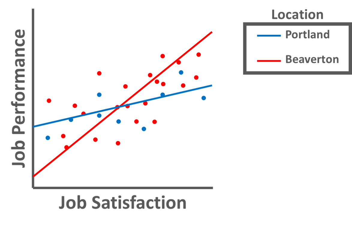
Moderators: A moderator (i.e., moderator variable) is a predictor variable upon which an association between two other variables is conditional. A moderator variable can be continuous (e.g., age: measured in years) or categorical (e.g., location: Portland vs. Beaverton). When we find that one variable moderates the association between two other variables, we often refer to this as an interaction or interaction effect. For example, let’s imagine that we are interested in the association between job satisfaction and job performance in our organization. By introducing the categorical moderator variable of employee location (Portland vs. Beaverton), we can determine whether the magnitude and/or sign of the association between job satisfaction and job performance varies by the location at which employees work. Perhaps we find that the association between job satisfaction and job performance is significantly stronger for employees who work in Beaverton as compared to employees who work in Portland (see figure below), and thus we would conclude that there is a significant interaction between job satisfaction and location in relation to job performance.
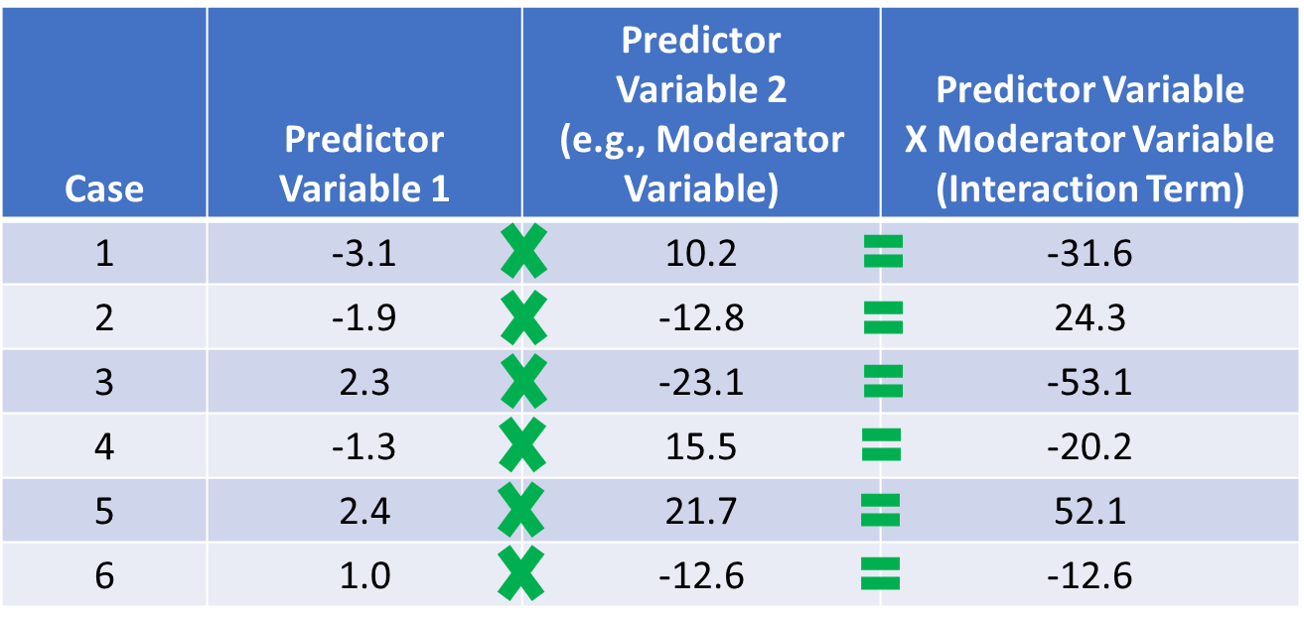
When investigating whether an interaction exists between two variables relative to the outcome variable, we need to create a new variable called an interaction term (i.e., product term). An interaction term is created by multiplying the scores of two predictor variables – or in other words, the computing the product of two variables’ respective scores. In fact, the presence of an in interaction term – and associated multiplication – signals why MMLR is referred to as a multiplicative model. In terms of the language we use to describe an interaction and the associated interaction term, we often refer to one of the predictor variables involved in an interaction as the moderator. For an illustration of how an interaction term is created, please refer to the table below.
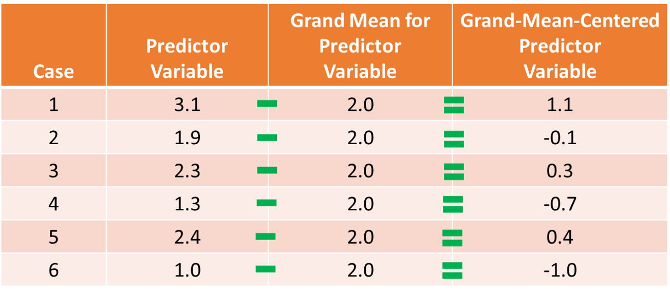
Centering Predictor & Moderator Variables: To improve the interpretability of the main effects (but not the interaction term) and to reduce collinearity between the predictor variables involved in the interaction term, we typically grand-mean center any continuous (interval, ratio) predictor variables; we do not need to center the outcome variable or a predictor or moderator variable that is categorical (e.g., dichotomous). As discussed in the chapter on centering and standardizing variables, grand-mean centering refers to the process of subtracting the overall sample mean for a variable from each case’s score on that variable. We center the predictor variables (i.e., predictor and moderator variables) before computing the interaction term based on those variables. To illustrate how grand-mean centering works, take a look at the table below, and note that we are just subtracting the (grand) mean for the sample from the specific value on the predictor variable for each case.
When we grand-mean center the predictor variables in a regression model, it also changes our interpretation of the \(\hat{Y}\)-intercept value. If you recall from prior reviews of simple linear regression and multiple linear regression, the \(\hat{Y}\)-intercept value is the mean of the outcome variable when each predictor variable(s) in the model is/are set to zero. Thus, when we center each predictor variable, we shift the mean of each variable to zero, which means that after grand-mean centering, the \(\hat{Y}\)-intercept value is the mean of the outcome variable when each predictor variable is set to its mean. Beyond moderated multiple linear regression, grand-mean centering can be useful in simple and multiple linear regression models when interpreting the regression coefficients associated with the intercept and the slope(s), as in some cases, a score of zero on the predictor variable is theoretically meaningless, implausible, or both. For example, if one of our predictor variables has an interval measurement scale that ranges from 10-100, then a score of zero is not even part of the scale range, which would make shifting the zero value to the grand-mean a more meaningful value.
Regardless of your decision to grand-mean center or to not grand-mean center the predictor variable and moderator variables, the interaction term’s significance level (p-value) and model fit (i.e., R2) will remain the same. In fact, sometimes it makes more sense to plot the findings of your model based on the uncentered version of the variables. That choice is really up to you and should be based on the context at hand.
Moderated Multiple Linear Regression: In moderated multiple linear regression (MMLR), we have three or more predictor variables and a single outcome variable, where one of the predictor variables is the interaction term (i.e., product term) between two of the predictor variables (e.g., predictor and moderator variables). Just like multiple linear regression, MMLR allows for a series of covariates (control variables) to be included in the model; accordingly, each regression coefficient (i.e., slope, weight) represents the relationship between the associated predictor and the outcome variable when statistically controlling for all other predictors in the model.
To better understand what MMLR is and how it works, I find that it’s useful to consider a MMLR model in equation form. Specifically, let’s consider a scenario in which we estimate a MMLR with two predictor variables, their interaction term (i.e., product term), and a single outcome variable. The equation for such a model with unstandardized regression coefficients (\(b\)) would be as follows:
\(\hat{Y} = b_{0} + b_{1}X_1 + b_{2}X_2 + b_{3}X_1*X_2 + e\)
where \(\hat{Y}\) represents the predicted score on the outcome variable (\(Y\)), \(b_{0}\) represents the \(\hat{Y}\)-intercept value (i.e., model constant) when the predictor variables \(X_1\) and \(X_2\) and interaction term \(X_1*X_2\) are equal to zero, \(b_{1}\), \(b_{2}\), and \(b_{3}\) represent the unstandardized coefficients (i.e., weights, slopes) of the associations between the predictor variables \(X_1\) and \(X_2\) and interaction term \(X_1*X_2\), respectively, and the outcome variable \(\hat{Y}\), and \(e\) represents the (residual) error in prediction. If the regression coefficient associated with the interaction term (\(b_{3}\)) is found to be statistically significant, then we would conclude that there is evidence of a significant interaction effect.
If we conceptualize one of the predictor variables as a moderator variable, then we might re-write the equation from above by swapping out \(X_2\) with \(W\) (or \(Z\)). The meaning of the equation remains the same, but changing the notation in this way may signal more clearly which variable we are labeling a moderator.
\(\hat{Y} = b_{0} + b_{1}X + b_{2}W + b_{3}X*W + e\)
Unstandardized regression coefficient indicates the “raw” regression coefficient (i.e., weight, slope) when controlling for the associations between all other predictors in the model and the outcome variable; accordingly, each unstandardized regression coefficient represents how many unstandardized units of \(\hat{Y}\) increase/decrease as a result of a single unit increase in a predictor variable, when statistically controlling for the effects of other predictors in the regression model.
Typically, we are most interested in whether slope differences exist; with that being said, in the context of testing for differential prediction (described below), we are also interested in whether intercept differences exist. In essence, a significant interaction term indicates the presence of slope differences, where slopes differences refer to significant variation in the association (i.e., slope) between the predictor variable and outcome variable by levels/values of the moderator variable. In the context of our first MMLR equation (see above), if the regression coefficient (\(b_{3}\)) associated with the interaction term (\(X_1*X_2\)) is statistically significant, we conclude that there is significant interaction and thus significant slope differences. In fact, we might even us language like, “\(X_2\) moderates the association between \(X_1\) and \(Y\).”
When we find a statistically significant interaction, it is customary to plot the simple slopes and estimate whether each of the simple slopes is significantly different from zero. Simple slopes allow us to probe the form of the significant interaction so that we can more accurately describe it. Plus, the follow-up simple slopes analysis helps us understand at which levels of the moderator variable the association between the predictor and outcome variables is statistically significant. For a continuous moderator variable, we typically plot and estimate the simple slopes at 1 standard deviation (SD) above and below the mean for the variable – and sometimes at the mean of the variable as well; with that being said, if we want, we can choose more theoretically or empirically meaningful values for the moderator variable. For a categorical variable, we plot and estimate the simple slopes based on the different discrete levels (categories) of the variable. For example, if our moderator variable captures gender identity operationalized as man (0) and woman (1), then we would plot the simple slopes when sex is equal to man (0) and when sex is equal to woman (1).
43.1.1.1 Statistical Assumptions
The statistical assumptions that should be met prior to running and/or interpreting estimates from a moderated multiple linear regression model are the same as those for conventional multiple linear regression include:
- Cases are randomly sampled from the population, such that the variable scores for one individual are independent of the variable scores of another individual;
- Data are free of multivariate outliers;
- The association between the predictor and outcome variables is linear;
- There is no (multi)collinearity between predictor variables;
- Average residual error value is zero for all levels of the predictor variables;
- Variances of residual errors are equal for all levels of the predictor variables, which is referred to as the assumption of homoscedasticity;
- Residual errors are normally distributed for all levels of the predictor variables.
The fourth statistical assumption refers to the concept of collinearity (multicollinearity). This can be a tricky concept to understand, so let’s take a moment to unpack it. When two or more predictor variables are specified in a regression model, as is the case with multiple linear regression, we need to be wary of collinearity. Collinearity refers to the extent to which predictor variables correlate with each other. Some level of intercorrelation between predictor variables is to be expected and is acceptable; however, if collinearity becomes substantial, it can affect the weights – and even the signs – of the regression coefficients in our model, which can be problematic from an interpretation standpoint. As such, we should avoid including predictors in a multiple linear regression model that correlate highly with one another. The tolerance statistic is commonly computed and serves as an indicator of collinearity. The tolerance statistic is computed by computing the shared variance (R2) of just the predictor variables in a single model (excluding the outcome variable), and subtracting that R2 value from 1 (i.e., 1 - R2). We typically grow concerned when the tolerance statistic falls below .20 and closer to .00. Ideally, we want the tolerance statistic to approach 1.00, as this indicates that there are lower levels of collinearity. From time to time, you might also see the variance inflation factor (VIF) reported as an indicator of collinearity; the VIF is just the reciprocal of the tolerance (i.e., 1/tolerance), and in my opinion, it is redundant to report and interpret both the tolerance and VIF. My recommendation is to focus just on the tolerance statistic when inferring whether the statistical assumption of no collinearity might have been violated.
Finally, with respect to the assumption that cases are randomly sampled from population, we will assume in this chapter’s data that this is not an issue. If we were to suspect, however, that there were some clustering or nesting of cases in units/groups (e.g., by supervisors, units, or facilities) with respect to our outcome variable, then we would need to run some type of multilevel model (e.g., hierarchical linear model, multilevel structural equation model), which is beyond the scope of this tutorial. An intraclass correlation (ICC) can be used to diagnose such nesting or cluster. Failing to account for clustering or nesting in the data can bias estimates of standard errors, which ultimately influences the p-values and inferences of statistical significance.
43.1.1.2 Statistical Signficance
Using null hypothesis significance testing (NHST), we interpret a p-value that is less than .05 (or whatever two- or one-tailed alpha level we set) to meet the standard for statistical significance, meaning that we reject the null hypothesis that the regression coefficient is equal to zero when controlling for the effects of the other predictor variable(s) and interaction term variable in the model. In other words, if a regression coefficient’s p-value is less than .05, we conclude that the regression coefficient differs from zero to a statistically significant extent when controlling for the effects of other predictor variables in the model. In contrast, if the regression coefficient’s p-value is equal to or greater than .05, then we fail to reject the null hypothesis that the regression coefficient is equal to zero when controlling for the effects of other predictor variable(s) and interaction term variable in the model. Put differently, if a regression coefficient’s p-value is equal to or greater than .05, we conclude that the regression coefficient does not differ from zero to a statistically significant extent, leading us to conclude that there is no association between the predictor variable (or interaction term variable) and the outcome variable in the population – when controlling for the effects of other predictor variables and interaction term variable in the model.
When setting an alpha threshold, such as the conventional two-tailed .05 level, sometimes the question comes up regarding whether borderline p-values signify significance or nonsignificance. For our purposes, let’s be very strict in our application of the chosen alpha level. For example, if we set our alpha level at .05, p = .049 would be considered statistically significant, and p = .050 would be considered statistically nonsignificant.
Because our regression model estimates are based on data from a sample that is drawn from an underlying population, sampling error will affect the extent to which our sample is representative of the population from which its drawn. That is, a regression coefficient estimate (b) is a point estimate of the population parameter that is subject to sampling error. Fortunately, confidence intervals can give us a better idea of what the true population parameter value might be. If we apply an alpha level of .05 (two-tailed), then the equivalent confidence interval (CI) is a 95% CI. In terms of whether a regression coefficient is statistically significant, if the lower and upper limits of 95% CI do not include zero, then this tells us the same thing as a p-value that is less than .05. Strictly speaking, a 95% CI indicates that if we were to hypothetically draw many more samples from the underlying population and construct CIs for each of those samples, then the true parameter (i.e., true value of the regression coefficient in the population) would likely fall within the lower and upper bounds of 95% of the estimated CIs. In other words, the 95% CI gives us an indication of plausible values for the population parameter while taking into consideration sampling error. A wide CI (i.e., large difference between the lower and upper limits) signifies more sampling error, and a narrow CI signifies less sampling error.
43.1.1.3 Practical Significance
As a reminder, an effect size is a standardized metric that can be compared across samples. In a moderated multiple linear regression (MMLR) model, an unstandardized regression coefficient (\(b\)) is not an effect size. The reason being, an unstandardized regression coefficient estimate is based on the original scaling of the predictor and outcome variables, and thus the same effect will take on different regression coefficients to the extent that the predictor and outcome variables have different scalings across samples.
A standardized regression coefficient (\(\beta\)) can be interpreted as an effect size (and thus an indicator of practical significance) given that it is standardized. With that being said, I suggest doing so with caution as collinearity (i.e., correlation) between predictor variables in the model can bias our interpretation of \(\beta\) as an effect size. Thus, if your goal is just to understand the bivariate association between a predictor variable and an outcome variable (without introducing statistical control), then I recommend to just estimate a correlation coefficient as an indicator of practical significance, which I discuss in the chapter on estimating criterion-related validity using correlations.
In a MMLR model, we can also describe the magnitude of the effect in terms of the proportion of variance explained in the outcome variable by the predictor variables (i.e., R2). That is, in a multiple linear regression model, R2 represents the proportion of collective variance explained in the outcome variable by all of the predictor variables. Conceptually, we can think of the overlap between the variability in the predictor variables and and outcome variable as the variance explained (R2), and R2 is a way to evaluate how well a model fits the data (i.e., model fit). I’ve found that the R2 is often readily interpretable by non-analytics audiences. For example, an R2 of .25 in a MMLR model can be interpreted as: the predictor variable and interaction term variable scores explain 25% of the variability in scores on the outcome variable. That is, to convert an R2 from a proportion to a percent, we just multiply by 100.
| R2 | Description |
|---|---|
| .01 | Small |
| .09 | Medium |
| .25 | Large |
43.1.2 Review of Differential Prediction
Differential prediction refers to differences in intercepts, slopes, or both based on subgroup (projected class) membership (Society for Industrial & Organizational Psychology 2018; Cleary 1968), and sometimes differential prediction is referred to as predictive bias. Assuming a single regression line is used to predict the criterion (e.g., job performance) scores of applicants, differential prediction is concerned with overpredicting or underpredicting criterion scores for one subgroup relative to another (Cascio and Aguinis 2005). A common regression line would be inappropriate when evidence of intercept differences, slope differences, or both exist.
In the U.S., the use of separate regression lines – one for each subgroup – is legally murky, with some interpreting separate regression lines as violation of federal law and others cautioning that the practice might be interpreted as score adjustment, thereby running afoul of the Civil Rights Act of 1991 (Berry 2015; Saad and Sackett 2002). Specifically, Section 106 of the Civil Rights Act of 1991 amends Section 703 of the Civil Rights Act of 1964 to prohibit the discriminatory use of selection test scores:
“It shall be an unlawful employment practice for a respondent, in connection with the selection or referral of applicants or candidates for employment or promotion, to adjust the scores of, use different cutoff scores for, or otherwise alter the results of, employment related tests on the basis of race, color, religion, sex, or national origin.”
Thus, a legally cautious approach would be to discontinue the use of a selection tool in its current form should evidence of differential prediction come to light.
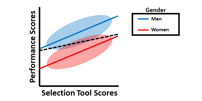
We’ll begin by considering an example of intercept differences when predicting scores on the criterion (e.g., job performance) based on scores on a selection tool. Imagine a situation in which scores on a selection tool differentially predict scores on job performance for men and women, such that the slopes are the same, but the intercepts of each slope are different (see figure below). The dashed black line indicates what a common regression line would look like if it were used. As you can see, if we were to use a single common regression line when intercept differences exist between men and women, then we would tend to underpredict job performance scores for men and overpredict for women.
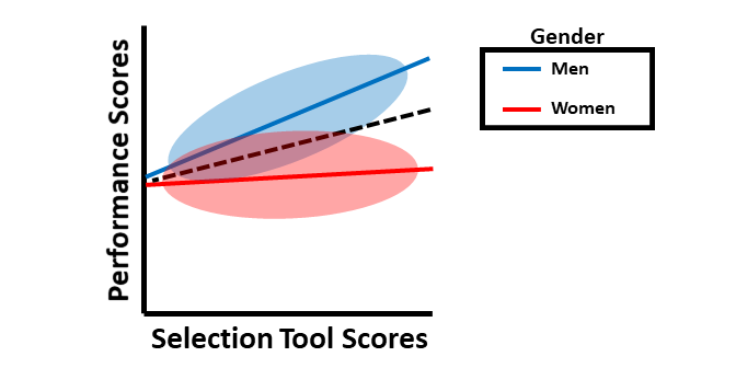
Next, we’ll consider an example involving slope differences in the context of differential prediction. In the figure below, the slopes (e.g., criterion-related validities) are different when the selection tool is used for men as compared to women. Again, the dashed black line represents what would happen if a common regression line were used, which would clearly be inappropriate. Note that, in this particular example, the job performance scores would generally be underpredicted for men and overpredicted for women when using the same regression. Further, the selection tool appears to show criterion-related validity (i.e., a significant slope) for men but not for women. Accordingly, based on this sample, the selection tool might only be a valid predictor of job performance for men. Clearly this would be a problem.
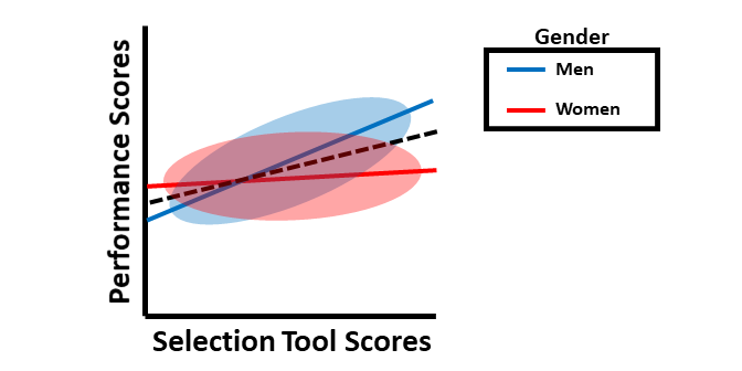
Finally, we’ll consider an example involving both intercept differences and slope differences. The figure below shows that use of a common regression line would pose problems in terms of predictive bias. In this example, for men, using of a common regression line would overpredict job performance scores for a certain range of selection tool scores and underpredict job performance scores for another range of selection tool scores; the opposite would be true for women.
Words of Caution: In this tutorial, we will learn how to apply MMLR in the service of detecting differential predication using an approach that is generally supported by the U.S. court system and researchers. With that said, using MMLR to detect differential prediction should be used cautiously with small samples, as failure to detect differential prediction that actually exists (i.e., Type II Error, false negative) could be the result of low statistical power, and relatedly, unreliability or bias in the selection tool or criterion and violation of certain statistical assumptions (e.g., homoscedasticity of residual error variances) can affect our ability to find differential prediction that actually exists (Aguinis and Pierce 1998). Further, when one subgroup is less than 30% of the total sample size, statistical power is also diminished (Stone-Romero, Alliger, and Aguinis 1994). The take-home message is to remain cautious and thoughtful when investigating differential prediction.
Multistep MMLR Process for Differential Prediction: We will use a three-step “step-up” process for investigating differential prediction using MMLR (Society for Industrial & Organizational Psychology 2018; Cleary 1968). This process uses what is referred to as hierarchical regression, as additional predictor variables are added at each subsequent step, and their incremental validity above and beyond the other predictors in the model is assessed.
In the first step, we will regress the criterion variable on the selection tool variable, and in this step, we will verify whether the selection tool shows criterion-related validity by itself. If we find evidence of criterion-related validity for the selection tool in this first step, then we proceed to the second and third steps.
In the second step, we include the selection tool variable as before but add the dichotomous (binary) protected class/group variable to the model. If the protected class variable is statistically significant when controlling for the selection tool variable, then there is evidence of intercept differences. You might be asking yourself: What happens when a protected class variable is not inherently categorical or, specifically, dichotomous? When it comes to the protected class of race, many organizations have more than two races represented among their employees. In this situation, it is customary (at least within the U.S.) to compare two subgroups at time (e.g., White and Black) or to create a dichotomy consisting of the majority race and members of other non-majority races (e.g., White and Non-White). For a inherently continuous variable like age, classically, the standard procedure was to dichotomize the age variable by those who are 40 years and older and those who are younger than 40 years, as this is consistent with the U.S. Age Discrimination in Employment Act (ADEA) of 1967. There are two potential issues with this: (a) Some states have further age protections in place that protect workers under 40 as well, and (b) Some jobs in organizations have very young workforces, leaving the question of whether people in their 30s are being favored over people in their 20s, or vice versa (for example). In addition, when we look at organizations with workers who are well into their 50s, 60s, and 70s, then there might be evidence of age discrimination and differential prediction for those who are in their 50s compared to those who are in their 60s. Dichotomizing the age variable using a 40 and above vs. under 40 split might miss these issues and generally nuance. (For a review of this topic, see Fisher et al. 2017.) As such, with a variable like age, there might be some advantages to keeping it as a continuous variable, as MMLR can handle this.
In the third step, we include the selection tool and protected class variables as before but add the interaction term between the selection tool and protected class variables. If the interaction term is statistically significant, then there is evidence of differential prediction in the form of slope differences.
43.1.2.1 Sample Write-Up
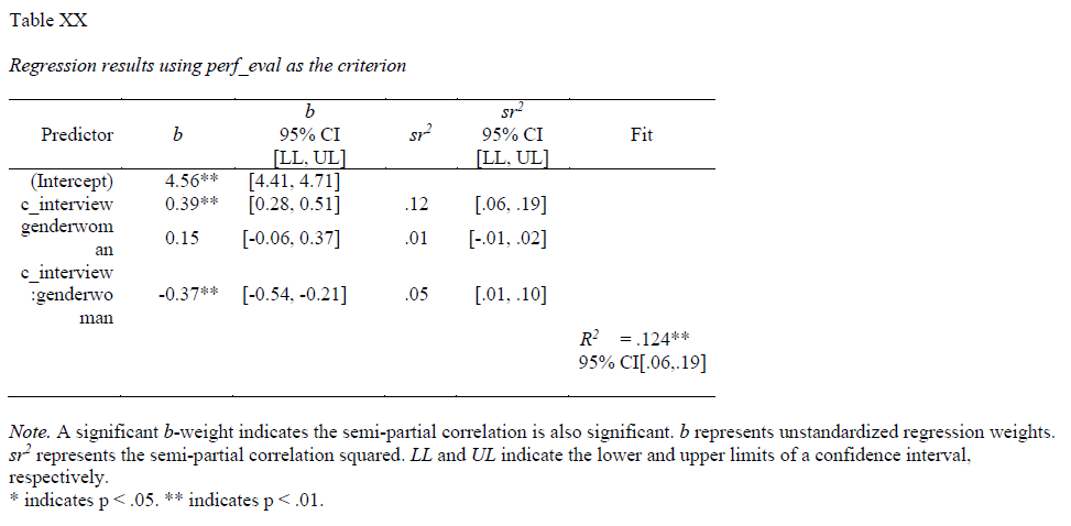
Our HR analytics team recently found evidence in support of the criterion-related validity of a new structured interview selection procedure. As a next step, we investigated whether there might be evidence of differential prediction for the structured interview based on the U.S. protected class of gender. Based on a sample of 370 individuals, we applied a three-step “step up” process with moderated multiple linear regression, which is consistent with established principles (Society for Industrial & Organizational Psychology 2018; Cleary 1968). Based on our analyses, we found evidence of differential prediction (i.e., predictive bias) based on gender for the new structured interview procedure, and specifically, we found evidence of slope differences. In the first step, we found evidence of criterion-related validity based on a simple linear regression model, as structured interview scores were positively and significantly associated with job performance (b = .192, p < .001), thereby indicating some degree of job-relatedness and -relevance. In the second step, we added the protected class variable associated with gender to the model, resulting in a multiple linear regression model, but we did not find evidence of intercept differences (b = .166, p = .146). In the third step, we added the interaction term between the structured interview and gender variables, resulting in a moderated multiple linear regression model, and we found that gender moderated the association between interview scores and job performance scores to a statistically significant extent (b = -.373, p < .001). Based on follow-up simple slopes analyses, we found that the association between structured interview scores and job performance scores was statistically significant and positive for men (b = .39, p < .01), such that for every one unit increase in structured interview scores, job performance scores tended to increase by .39 units; in contrast, the association between structured interview scores and job performance scores for women was nonsignificant (b = .02, p = .72). In sum, we found evidence of slope differences, which means that this interview tool shows evidence of predictive bias with respect to gender, making the application of a common regression line (i.e., equation) egally problematic within the United States. If possible, this structured interview should be redesigned or the interviewers should be trained to reduce the predictive bias based on gender. In the interim, we caution against using separate regression lines for men and women, as this may be interpreted as running afoul of the U.S. Civil Rights Act of 1991 (Saad and Sackett 2002). A more conservative approach would be to develop a structured interview process that allows for the use of a common regression line across legally protected groups.
43.2 Tutorial
This chapter’s tutorial demonstrates how to use moderated multiple linear regression in the service of detecting differential prediction in a selection tool.
43.2.1 Video Tutorial
As usual, you have the choice to follow along with the written tutorial in this chapter or to watch the video tutorial below.
Link to video tutorial: https://youtu.be/3n2vvMc4yHs
43.2.2 Functions & Packages Introduced
| Function | Package |
|---|---|
mean |
base R |
Regression |
lessR |
reg_brief |
lessR |
probe_interaction |
interactions |
43.2.3 Initial Steps
If you haven’t already, save the file “DifferentialPrediction.csv” into a folder that you will subsequently set as your working directory. Your working directory will likely be different than the one shown below (i.e., "H:/RWorkshop"). As a reminder, you can access all of the data files referenced in this book by downloading them as a compressed (zipped) folder from the my GitHub site: https://github.com/davidcaughlin/R-Tutorial-Data-Files; once you’ve followed the link to GitHub, just click “Code” (or “Download”) followed by “Download ZIP”, which will download all of the data files referenced in this book. For the sake of parsimony, I recommend downloading all of the data files into the same folder on your computer, which will allow you to set that same folder as your working directory for each of the chapters in this book.
Next, using the setwd function, set your working directory to the folder in which you saved the data file for this chapter. Alternatively, you can manually set your working directory folder in your drop-down menus by going to Session > Set Working Directory > Choose Directory…. Be sure to create a new R script file (.R) or update an existing R script file so that you can save your script and annotations. If you need refreshers on how to set your working directory and how to create and save an R script, please refer to Setting a Working Directory and Creating & Saving an R Script.
Next, read in the .csv data file “DifferentialPrediction.csv” using your choice of read function. In this example, I use the read_csv function from the readr package (Wickham, Hester, and Bryan 2024). If you choose to use the read_csv function, be sure that you have installed and accessed the readr package using the install.packages and library functions. Note: You don’t need to install a package every time you wish to access it; in general, I would recommend updating a package installation once ever 1-3 months. For refreshers on installing packages and reading data into R, please refer to Packages and Reading Data into R.
# Install readr package if you haven't already
# [Note: You don't need to install a package every
# time you wish to access it]
install.packages("readr")
# Access readr package
library(readr)
# Read data and name data frame (tibble) object
DiffPred <- read_csv("DifferentialPrediction.csv")## Rows: 320 Columns: 6
## ── Column specification ────────────────────────────────────────────────────────────────────────────────────────────────────────────
## Delimiter: ","
## chr (3): emp_id, gender, race
## dbl (3): perf_eval, interview, age
##
## ℹ Use `spec()` to retrieve the full column specification for this data.
## ℹ Specify the column types or set `show_col_types = FALSE` to quiet this message.## [1] "emp_id" "perf_eval" "interview" "gender" "age" "race"## spc_tbl_ [320 × 6] (S3: spec_tbl_df/tbl_df/tbl/data.frame)
## $ emp_id : chr [1:320] "EE200" "EE202" "EE203" "EE206" ...
## $ perf_eval: num [1:320] 6.2 6.6 5 4 5.3 5.9 5.5 3.8 5.7 3.8 ...
## $ interview: num [1:320] 8.5 5.7 7 6.8 9.6 6 7.5 5.9 9.6 8.3 ...
## $ gender : chr [1:320] "woman" "woman" "man" "woman" ...
## $ age : num [1:320] 30 45.6 39.2 36.9 24.5 41.5 35.1 43.2 25.7 27.8 ...
## $ race : chr [1:320] "black" "black" "asian" "black" ...
## - attr(*, "spec")=
## .. cols(
## .. emp_id = col_character(),
## .. perf_eval = col_double(),
## .. interview = col_double(),
## .. gender = col_character(),
## .. age = col_double(),
## .. race = col_character()
## .. )
## - attr(*, "problems")=<externalptr>## # A tibble: 6 × 6
## emp_id perf_eval interview gender age race
## <chr> <dbl> <dbl> <chr> <dbl> <chr>
## 1 EE200 6.2 8.5 woman 30 black
## 2 EE202 6.6 5.7 woman 45.6 black
## 3 EE203 5 7 man 39.2 asian
## 4 EE206 4 6.8 woman 36.9 black
## 5 EE209 5.3 9.6 woman 24.5 white
## 6 EE214 5.9 6 woman 41.5 asianThere are 6 variables and 370 cases (i.e., employees) in the DiffPred data frame: emp_id, perf_eval, interview, age, gender, and race. Per the output of the str (structure) function above, the variables perf_eval, interview, and age are of type numeric (continuous: interval/ratio), and the variables emp_id, gender, and race are of type character (nominal/categorical). The variable emp_id is the unique employee identifier. Imagine that these data were collected as part of a criterion-related validation study - specifically, a concurrent validation design in which job incumbents were administered a rated structured interview (interview) 90 days after entering the organization. The structured interview (interview) variable was designed to assess individuals’ interpersonal skills, and ratings can range from 1 (very weak interpersonal skills) to 10 (very strong interpersonal skills). The interviews were scored by untrained raters who were often the hiring managers but not always. The perf_eval variable is the criterion (outcome) of interest, and it is a 90-day-post-hire measure of supervisor-rated job performance, with possible ratings ranging from 1-7, with 7 indicating high performance. The age variable represents the job incumbents’ ages (in years). The gender variable represents the job incumbents’ tender identify and is defined by two levels/categories/values: man and woman. Finally, the race variable represents the job incumbents’ race/ethnicity and is defined by three levels/categories/values: asian, black, and white.
43.2.4 Grand-Mean Center Continuous Predictor Variables
To improve the interpretability of our model and to reduce the collinearity between the predictor and moderator variables with their interaction term, we will grand-mean center continuous predictor and moderator variables. [Note: A moderator variable is just a predictor variable that we are framing as a moderator.] With regard to interpretability, grand-mean centering aids in our interpretation of the regression coefficients associated with our predictor and moderator variables in our MMLR by reducing collinearity between these variables and their interaction term and by estimating the y-intercept when all predictors are at their respective means (averages), as opposed to when they are at zero (which is not always a plausible or meaningful value for some variables). Further, when interpreting the association between one predictor variable and the outcome variable while statistically controlling for other variables in the model, grand-mean centering allows us to interpret the effect of the focal predictor variable when the other predictor variables are at their respective means (as opposed to zero). For more detailed information on centering, check out the chapter on centering and standardizing variables.
We only center predictor and moderator variables that are of type numeric and that we conceptualize as having a continuous (interval or ratio) measurement scale. In our current data frame, we will grand-mean center just the interview and age variables. We will use what is perhaps the most intuitive approach for grand-mean centering variables. We must begin by coming up with a new name for one of our soon-to-be grand-mean centered variable, and in this example, we will center the interview variable. I typically like to name the centered variable by simply adding the c_ prefix to the existing variable’s names (e.g., c_interview). Type the name of the data frame object to which the new centered variable will be attached (DiffPred), followed by the $ operator and the name of the new variable we are creating (c_interview). Next, add the <- operator to indicate what values you will assign to this new variable. To create a vector of values to assign to this new c_interview variable, we will subtract the mean (average) score for the original variable (interview) from each case’s value on the variable. Specifically, enter the name of the data frame object, followed by the $ operator and the name of the original variable (interview). After that, enter the subtraction operator (-). And finally, type the name of the mean function from base R. As the first argument in the mean function, enter the name of the data frame object (DiffPred), followed by the $ operator and the name of the original variable (interview). As the second argument, enter na.rm=TRUE to indicate that you wish to drop missing values when calculating the grand mean for the sample. Now repeat those same steps for the age variable.
43.2.5 Estimate Moderated Multiple Linear Regression Model
As described above, we will use the standard three-step differential prediction assessment using MMLR. We will repeat this three step process for all three protected class variables in our data frame: gender, c_age, and race. [Note that we are using the grand-mean centered age variable we created above.]. Our selection tool of interest is our c_interview (which is the grand-mean centered version of the variable we created above), and our criterion of interest is perf_eval. I will show you how to test differential prediction for each of these protected class variables using the Regression (or reg_brief) function from lessR (Gerbing, Business, and University 2021).
Note: To reduce the overall length of this tutorial, I have omitted the diagnostic tests of the statistical assumptions, and thus for the purposes of this tutorial, we will assume that the statistical assumptions have been met. For your own work, be sure to run diagnostic tests to evaluate whether your model meets these statistical assumptions. For more information on statistical assumption testing in this context, check out the chapter on estimating increment validity using multiple linear regression.
If you haven’t already install and access the lessR package using the install.packages and library functions, respectively (see above). This will allow us to access the Regression and reg_brief functions.
43.2.5.1 Test Differential Prediction Based on gender
Let’s start with investigating whether differential prediction exists for our interview selection tool in relation to perf_eval based gender subgroup membership (i.e., man, woman).
Step One: Let’s being by regressing the criterion variable perf_eval on the selection tool variable c_interview. Here we are just establishing whether the selection tool shows evidence of criterion-related validity. See the chapters on predicting criterion scores using simple linear regression if you would like more information on regression-based approaches to assessing criterion-related validity, including determining whether statistical assumptions have been met. You can use either the Regression or reg_brief function from lessR, where the latter provides less output. To keep the amount of output in this tutorial to a minimum, I will use the reg_brief function, but when you evaluate whether statistical assumptions have been met, be sure to use the full Regression function.
# Regress perf_eval (criterion) on c_interview (selection tool)
reg_brief(perf_eval ~ c_interview, data=DiffPred)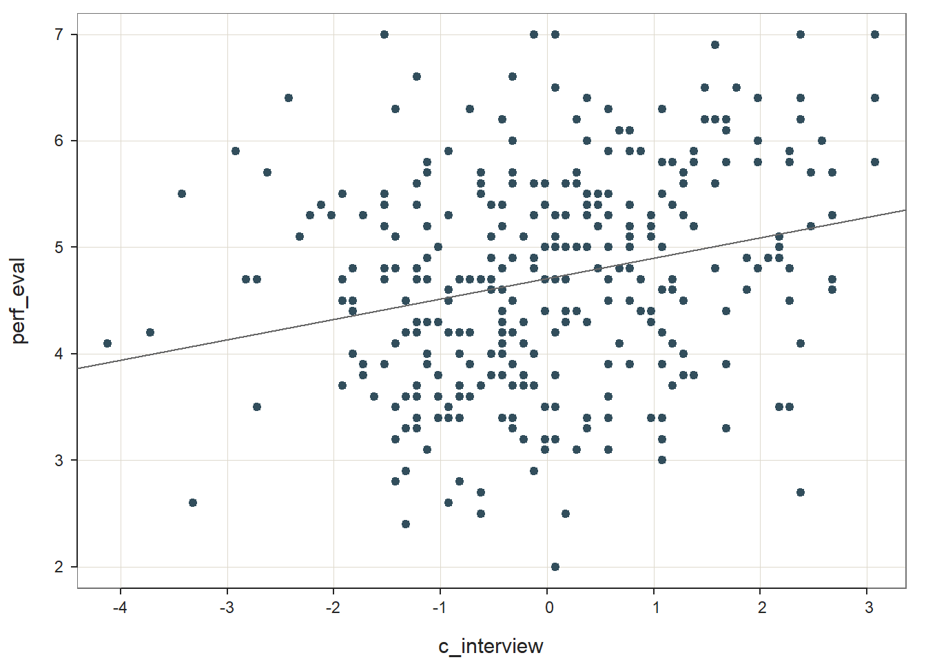
## >>> Suggestion
## # Create an R markdown file for interpretative output with Rmd = "file_name"
## reg(perf_eval ~ c_interview, data=DiffPred, Rmd="eg")
##
##
## BACKGROUND
##
## Data Frame: DiffPred
##
## Response Variable: perf_eval
## Predictor Variable: c_interview
##
## Number of cases (rows) of data: 320
## Number of cases retained for analysis: 320
##
##
## BASIC ANALYSIS
##
## Estimate Std Err t-value p-value Lower 95% Upper 95%
## (Intercept) 4.708 0.054 86.472 0.000 4.600 4.815
## c_interview 0.192 0.041 4.629 0.000 0.110 0.273
##
## Standard deviation of perf_eval: 1.005
##
## Standard deviation of residuals: 0.974 for 318 degrees of freedom
## 95% range of residual variation: 3.832 = 2 * (1.967 * 0.974)
##
## R-squared: 0.063 Adjusted R-squared: 0.060 PRESS R-squared: 0.051
##
## Null hypothesis of all 0 population slope coefficients:
## F-statistic: 21.425 df: 1 and 318 p-value: 0.000
##
## -- Analysis of Variance
##
## df Sum Sq Mean Sq F-value p-value
## Model 1 20.319 20.319 21.425 0.000
## Residuals 318 301.583 0.948
## perf_eval 319 321.902 1.009
##
##
## K-FOLD CROSS-VALIDATION
##
##
## RELATIONS AMONG THE VARIABLES
##
##
## RESIDUALS AND INFLUENCE
##
##
## PREDICTION ERRORThe unstandardized regression coefficient for c_interview is statistically significant and positive (b = .192, p < .001), which provides evidence of criterion-related validity. The amount of variance explained by c_interview in perf_eval is small-medium in magnitude (R2 = .063, adjusted R2 = .060, p < .001); that is, approximately 6% of the variability in perf_eval can be explained by c_interview. See the table below for common rules of thumbs for qualitatively describing R2 values.
| R2 | Description |
|---|---|
| .01 | Small |
| .09 | Medium |
| .25 | Large |
Because Step One revealed a statistically significant association between c_interview and perf_eval – and thus evidence of criterion-related validity for the selection tool – we will proceed to Step Two and Step Three. Had we not found evidence of criterion-related validity in Step One, we would have stopped at that step; after all, it won’t be worthwhile to look for evidence of differential prediction if we won’t be using the selection tool moving forward (given that it’s not job related).
Step Two: Next, let’s add the protected class variable gender to our model to investigate whether intercept differences exist. For more information on how to interpret and test the statistical assumptions of a multiple linear regression model, check out the chapter on estimating incremental validity using multiple linear regression. Note that this model can be called an additive model.
# Regress perf_eval (criterion) on c_interview (selection tool) and protected class (gender)
reg_brief(perf_eval ~ c_interview + gender, data=DiffPred)##
## >>> gender is not numeric. Converted to indicator variables.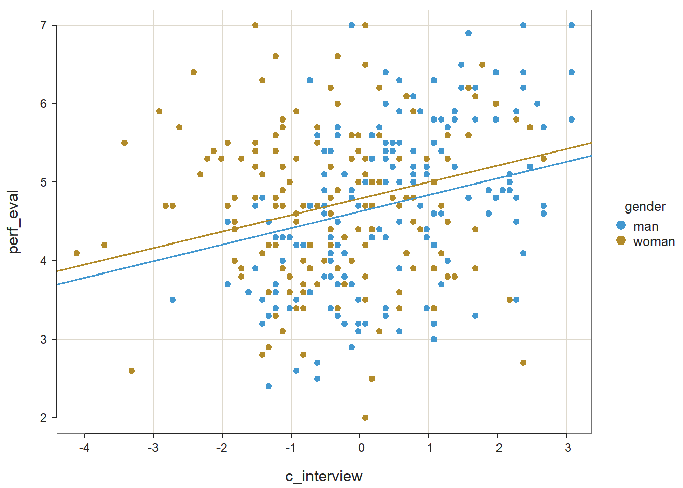
## >>> Suggestion
## # Create an R markdown file for interpretative output with Rmd = "file_name"
## reg(perf_eval ~ c_interview + gender, data=DiffPred, Rmd="eg")
##
##
## BACKGROUND
##
## Data Frame: DiffPred
##
## Response Variable: perf_eval
## Predictor Variable 1: c_interview
## Predictor Variable 2: genderwoman
##
## Number of cases (rows) of data: 320
## Number of cases retained for analysis: 320
##
##
## BASIC ANALYSIS
##
## Estimate Std Err t-value p-value Lower 95% Upper 95%
## (Intercept) 4.630 0.076 60.719 0.000 4.480 4.780
## c_interview 0.211 0.043 4.861 0.000 0.125 0.296
## genderwoman 0.166 0.114 1.458 0.146 -0.058 0.391
##
## Standard deviation of perf_eval: 1.005
##
## Standard deviation of residuals: 0.972 for 317 degrees of freedom
## 95% range of residual variation: 3.825 = 2 * (1.967 * 0.972)
##
## R-squared: 0.069 Adjusted R-squared: 0.063 PRESS R-squared: NA
##
## Null hypothesis of all 0 population slope coefficients:
## F-statistic: 11.813 df: 2 and 317 p-value: 0.000
##
## -- Analysis of Variance from Type II Sums of Squares
##
## df Sum Sq Mean Sq F-value p-value
## c_interview 1 22.328 22.328 23.626 0.000
## genderwoman 1 2.009 2.009 2.125 0.146
## Residuals 317 299.574 0.945
##
## -- Test of Interaction
##
## c_interview:gender df: 1 df resid: 316 SS: 17.514 F: 19.622 p-value: 0
##
## -- Assume parallel lines, no interaction of gender with c_interview
##
## Level man: y^_perf_eval = 4.630 + 0.211(x_c_interview)
## Level woman: y^_perf_eval = 4.796 + 0.211(x_c_interview)
##
## -- Visualize Separately Computed Regression Lines
##
## Plot(c_interview, perf_eval, by=gender, fit="lm")
##
##
## K-FOLD CROSS-VALIDATION
##
##
## RELATIONS AMONG THE VARIABLES
##
##
## RESIDUALS AND INFLUENCE
##
##
## PREDICTION ERRORThe unstandardized regression coefficient associated with gender (or more specifically genderwoman) is not statistically significant (b = .166, p = .146) when controlling for c_interview, which indicates that there is no evidence of intercept differences. Note that the name of the regression coefficient for gender has woman appended to it; this means that the intercept represents the perf_eval scores of women minus those for men. Behind the scenes, the reg_brief function has converted the gender variable to a dichotomous factor, where alphabetically man becomes 0 and woman becomes 1. Because the coefficient is negative, it implies that the intercept value is higher for women relative to men; however, please note that we wouldn’t interpret the direction of this effect because it was not statistically significant. The amount of variance explained by c_interview and gender in perf_eval is small-medium in magnitude (R2 = .069, adjusted R2 = .063, p < .001), which is slightly larger than when just c_interview was included in the model (see Step One above).
Because there is no evidence of intercept differences for Step Two, we won’t plot/graph the our model, as doing so might mislead someone who sees such a plot without knowing or understanding the results of the model we just estimated. We will now proceed to Step Three.
Step Three: As the final step, it’s time to add the interaction term (also known as a product term) between c_interview and gender to the model, which creates what is referred to as a multiplicative model. Fortunately, this is very easy to do in R. All we need to do is change the + operator from our previous regression model script to the *, where the * implies an interaction in the context of a model. Conceptually, the * is appropriate because we are estimating a multiplicative model containing an interaction term.
# Regress perf_eval (criterion) on c_interview (selection tool), protected class (gender),
# and interaction between selection tool and protected class
reg_brief(perf_eval ~ c_interview * gender, data=DiffPred)##
## >>> gender is not numeric. Converted to indicator variables.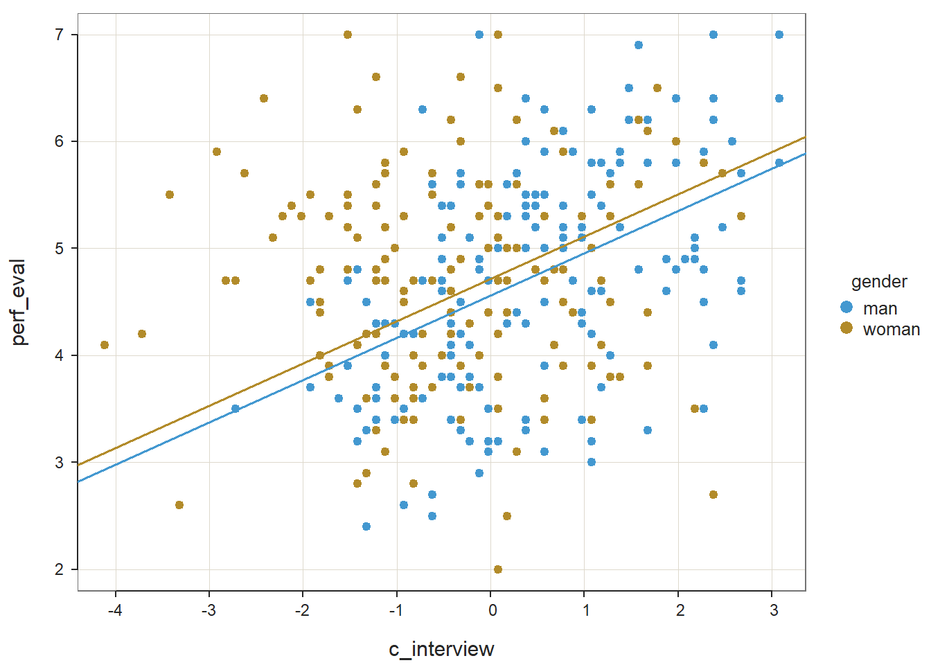
## >>> Suggestion
## # Create an R markdown file for interpretative output with Rmd = "file_name"
## reg(perf_eval ~ c_interview * gender, data=DiffPred, Rmd="eg")
##
##
## BACKGROUND
##
## Data Frame: DiffPred
##
## Response Variable: perf_eval
## Predictor Variable 1: c_interview
## Predictor Variable 2: genderwoman
## Predictor Variable 3: c_interview.genderwoman
##
## Number of cases (rows) of data: 320
## Number of cases retained for analysis: 320
##
##
## BASIC ANALYSIS
##
## Estimate Std Err t-value p-value Lower 95% Upper 95%
## (Intercept) 4.562 0.076 60.298 0.000 4.413 4.711
## c_interview 0.394 0.059 6.672 0.000 0.278 0.511
## genderwoman 0.155 0.111 1.397 0.163 -0.063 0.373
## c_interview.genderwoman -0.373 0.084 -4.430 0.000 -0.539 -0.207
##
## Standard deviation of perf_eval: 1.005
##
## Standard deviation of residuals: 0.945 for 316 degrees of freedom
## 95% range of residual variation: 3.718 = 2 * (1.967 * 0.945)
##
## R-squared: 0.124 Adjusted R-squared: 0.115 PRESS R-squared: NA
##
## Null hypothesis of all 0 population slope coefficients:
## F-statistic: 14.879 df: 3 and 316 p-value: 0.000
##
## -- Analysis of Variance from Type II Sums of Squares
##
## df Sum Sq Mean Sq F-value p-value
## c_interview 1 22.328 22.328 23.626 0.000
## genderwoman 1 2.009 2.009 2.250 0.135
## c_interview.genderwoman 1 17.514 17.514 19.622 0.000
## Residuals 316 282.060 0.893
##
## -- Test of Interaction
##
## c_interview:gender df: 1 df resid: 316 SS: 17.514 F: 19.622 p-value: 0
##
## -- Assume parallel lines, no interaction of gender with c_interview
##
## Level man: y^_perf_eval = 4.562 + 0.394(x_c_interview)
## Level woman: y^_perf_eval = 4.717 + 0.394(x_c_interview)
##
## -- Visualize Separately Computed Regression Lines
##
## Plot(c_interview, perf_eval, by=gender, fit="lm")
##
##
## K-FOLD CROSS-VALIDATION
##
##
## RELATIONS AMONG THE VARIABLES
##
##
## RESIDUALS AND INFLUENCE
##
##
## PREDICTION ERRORIn our output, we now have an unstandardized regression coefficient called c_interview:gender (or c_interview.gender), which represents our interaction term for c_interview and gender. The regression coefficient associated with the interaction term (c_interview:gender) is negative and statistically significant (b = -.373, p < .001), but we shouldn’t pay too much attention to the sign of the interaction term as it is difficult to interpret it without graphing the regression model in its entirety. We should, however, pay attention to the fact that the interaction term is statistically significant, which indicates that there is evidence of slope differences; in other words, there seems to be multiplicative effect between c_interview and gender. Although we didn’t find evidence of intercept differences in Step Two, here in Step Three, we do find evidence that the criterion-related validities for the selection tool (c_interview) in relation to the criterion (perf_eval) are significantly different from one another; in other words, we found evidence that the slopes for men and women differ. The amount of variance explained by c_interview, gender, and their interaction in relation to perf_eval is medium in magnitude (R2 = .124, adjusted R2 = .115, p < .001), which is larger than when just c_interview and gender were included in the model (see Step Two above).
Given the statistically significant interaction term, it is appropriate (and helpful) to probe the interaction by plotting it. This will help us understand the form of the interaction. We can do so by creating a plot of the simple slopes. To do so, we will use a package called interactions (Long 2019), so if you haven’t already, install and access the package.
# Install interactions package if you haven't already
install.packages("interactions")
# Note: You may need to install the sandwich package independently if you
# receive an error when attempting to run the probe_interaction function
# install.packages("sandwich")As input to the probe_interaction function from the interactions package, we will need to use the lm function base R to specify the same regression model we estimated above. We can just copy and paste the same arguments from the reg_brief function into the lm function parentheses. We need to name this model something so that we can reference it in the next function, so let’s name it Slope_Model (for slope differences model) using the <- operator.
# Regress perf_eval (criterion) on c_interview (selection tool), protected class (gender),
# and interaction between selection tool and protected class
Slope_Model <- lm(perf_eval ~ c_interview * gender, data=DiffPred)Now we’re ready to apply the probe_interaction in order to plot this multiplicative model. As the first argument, enter the name of the regression model we just created above (Slope_Model). As the second argument, type the name of the variable you are framing as the predictor after pred=, which in our case is the selection tool variable (c_interview). As the third argument, type the name of the variable you are framing as the moderator after modx=, which in our case is the protected class variable (gender). As the fourth argument, enter johnson_neyman=FALSE, as we aren’t requesting the Johnson-Neyman test in this tutorial. Finally, if you choose to, you can use x.label= and y.label= to create more informative names for the predictor and outcome variables, respectively. You could also add, if you should choose to do so, the legend.main= argument to provide a more informative name for the moderator variable, and/or the modx.labels= to provide more informative names for the moderator variable labels.
# Probe the significant interaction (slope differences)
probe_interaction(Slope_Model,
pred=c_interview,
modx=gender,
johnson_neyman=FALSE,
x.label="Interview Score",
y.label="Job Performance")## SIMPLE SLOPES ANALYSIS
##
## Slope of c_interview when gender = man:
##
## Est. S.E. t val. p
## ------ ------ -------- ------
## 0.39 0.06 6.67 0.00
##
## Slope of c_interview when gender = woman:
##
## Est. S.E. t val. p
## ------ ------ -------- ------
## 0.02 0.06 0.35 0.72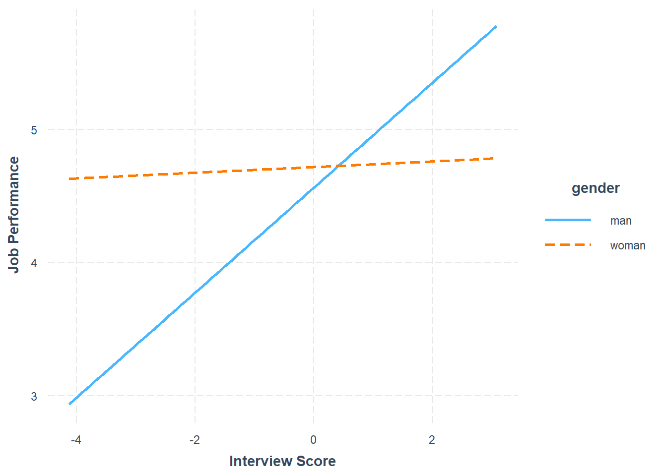
The plot output shows that the two slopes are indeed different, such that there doesn’t seem to be much of an association between the selection tool (c_interview) and the criterion (perf_eval) for women, but there seems to be a positive association for men. Now take a look at the text output in your console. The simple slopes analysis automatically estimates the regression coefficient (slope) for both levels of the moderator variable (gender: man, woman). Corroborating what we see in the plot, we find that the simple slope for men is indeed statistically significant and positive (b = .39, p < .01), such that for every one unit increase in interview scores, job performance scores tend to go up by .39 units. In contrast, we find that the simple slope for women is nonsignificant (b = .02, p = .72).
In sum, we found evidence of slope differences – but not intercept differences – for the selection tool (c_interview) in relation to the criterion (perf_eval) that were conditional upon the levels/subgroups of the protected class variable (gender). Thus, we can conclude that there is evidence of differential prediction based on gender for this interview selection tool, which means that it would be inappropriate to use a common regression line when predicting scores on the criterion based on the interview selection tool.
Sample Write-Up: Our HR analytics team recently found evidence in support of the criterion-related validity of a new structured interview selection procedure. As a next step, we investigated whether there might be evidence of differential prediction of the structured interview based on the U.S. protected class of gender. Based on a sample of 370 individuals, we applied a three-step process with moderated multiple linear regression, which is consistent with established principles (Society for Industrial & Organizational Psychology 2018; Cleary 1968). Based on our analyses, we found evidence differential prediction (i.e., predictive bias) based on gender for the new structured interview procedure, and specifically, we found evidence of slope differences. In the first step, we found evidence of criterion-related validity based on a simple linear regression model, as structured interview scores were positively and significantly associated with job performance (b = .192, p < .001), thereby indicating some degree of job-relatedness and -relevance. In the second step, we added the protected class variable associated with gender to the model, resulting in a multiple linear regression model, but did not find evidence of intercept differences based on gender (b = .166, p = .146). In the third step, we added the interaction term between the structured interview and gender variables, resulting in a moderated multiple linear regression model, and we found that gender moderated the association between structured interview scores and job performance scores to a statistically significant extent (b = -.373, p < .001). Based on follow-up simple slopes analyses, we found that the association between structured interview scores and job performance scores was statistically significant for men (b = .39, p < .01), such that for every one unit increase in structured interview scores, job performance scores tended to increase by .39 units; in contrast, the associated between structured interview scores and job performance scores for women was nonsignificant (b = .02, p = .72). In sum, we found evidence slope differences, which means that this structured interview tool shows predictive bias with respect to gender, making the application of a common regression line (i.e., equation) legally problematic within the United States. If possible, this structured interview should be redesigned or the interviewers should be trained to reduce the predictive bias based on gender. In the interim, we caution against using separate regression lines for men and women, as this may be interpreted as running afoul of the U.S. Civil Rights Act of 1991 (Saad and Sackett 2002). A more conservative approach would be to develop a structured interview process that allows for the use of a common regression line across legally protected groups.
43.2.5.2 Test Differential Prediction Based on c_age
Investigating whether differential prediction exists for c_interview in relation to perf_eval based on the continuous moderator variable c_age will unfold very similarly to the process we used for the dichotomous gender variable from above. The only differences will occur when it comes to estimating and visualizing the intercept differences and simple slopes (assuming we find statistically significant effects). Given this, we will breeze through the steps, which means I will provide less explanation.
Step One: Regress the criterion variable perf_eval on the selection tool variable c_interview.
# Regress perf_eval (criterion) on c_interview (selection tool)
reg_brief(perf_eval ~ c_interview, data=DiffPred)
## >>> Suggestion
## # Create an R markdown file for interpretative output with Rmd = "file_name"
## reg(perf_eval ~ c_interview, data=DiffPred, Rmd="eg")
##
##
## BACKGROUND
##
## Data Frame: DiffPred
##
## Response Variable: perf_eval
## Predictor Variable: c_interview
##
## Number of cases (rows) of data: 320
## Number of cases retained for analysis: 320
##
##
## BASIC ANALYSIS
##
## Estimate Std Err t-value p-value Lower 95% Upper 95%
## (Intercept) 4.708 0.054 86.472 0.000 4.600 4.815
## c_interview 0.192 0.041 4.629 0.000 0.110 0.273
##
## Standard deviation of perf_eval: 1.005
##
## Standard deviation of residuals: 0.974 for 318 degrees of freedom
## 95% range of residual variation: 3.832 = 2 * (1.967 * 0.974)
##
## R-squared: 0.063 Adjusted R-squared: 0.060 PRESS R-squared: 0.051
##
## Null hypothesis of all 0 population slope coefficients:
## F-statistic: 21.425 df: 1 and 318 p-value: 0.000
##
## -- Analysis of Variance
##
## df Sum Sq Mean Sq F-value p-value
## Model 1 20.319 20.319 21.425 0.000
## Residuals 318 301.583 0.948
## perf_eval 319 321.902 1.009
##
##
## K-FOLD CROSS-VALIDATION
##
##
## RELATIONS AMONG THE VARIABLES
##
##
## RESIDUALS AND INFLUENCE
##
##
## PREDICTION ERRORThe regression coefficient for c_interview is statistically significant and positive (b = .192, p < .001), which provides evidence of criterion-related validity. The amount of variance explained by c_interview in perf_eval is small-medium in magnitude (R2 = .063, adjusted R2 = .060, p < .001).
Step Two: Regress the criterion variable perf_eval on the selection tool variable c_interview and the protected class variable c_age.
# Regress perf_eval (criterion) on c_interview (selection tool) and protected class (c_age)
reg_brief(perf_eval ~ c_interview + c_age, data=DiffPred)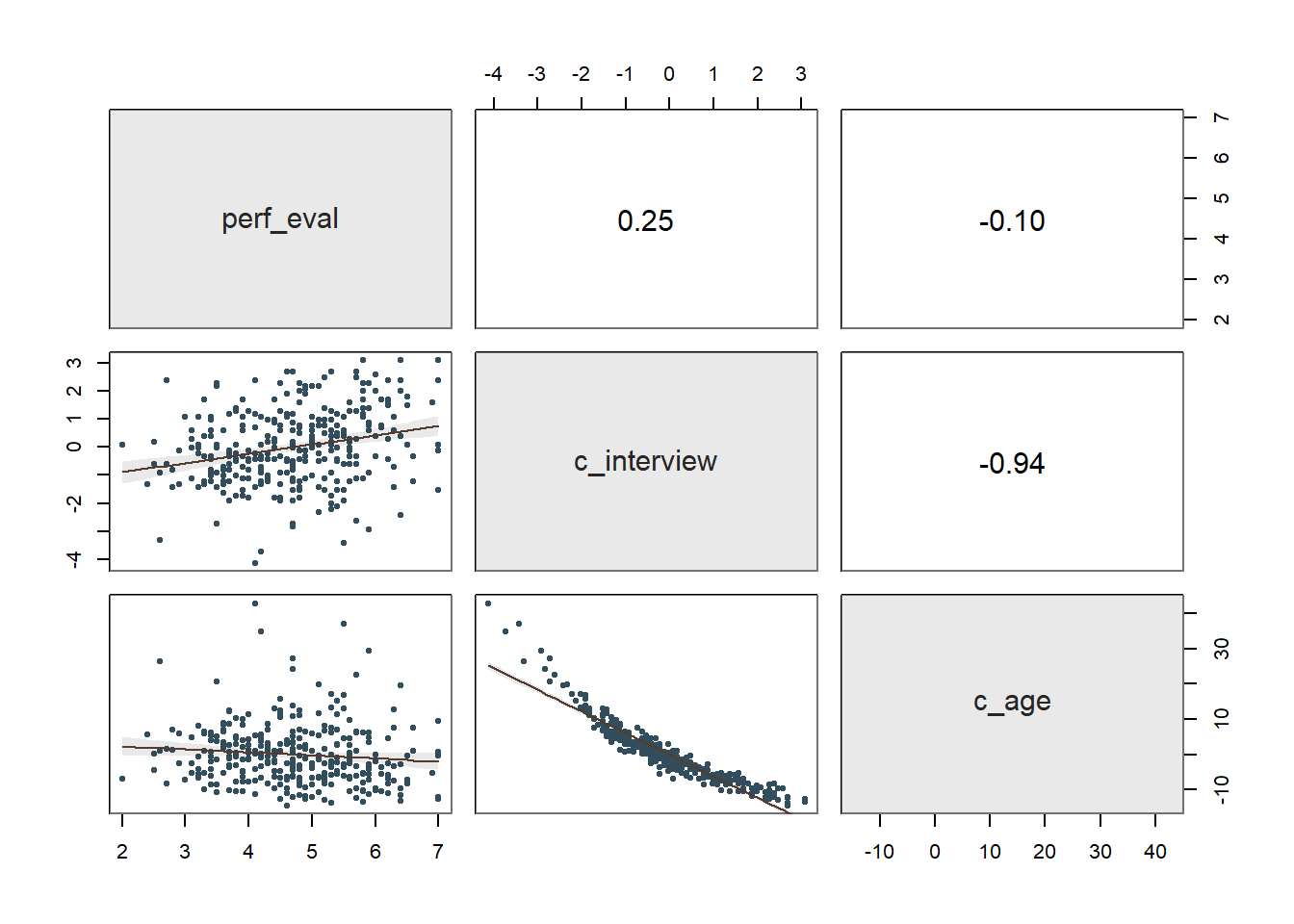
## >>> Suggestion
## # Create an R markdown file for interpretative output with Rmd = "file_name"
## reg(perf_eval ~ c_interview + c_age, data=DiffPred, Rmd="eg")
##
##
## BACKGROUND
##
## Data Frame: DiffPred
##
## Response Variable: perf_eval
## Predictor Variable 1: c_interview
## Predictor Variable 2: c_age
##
## Number of cases (rows) of data: 320
## Number of cases retained for analysis: 320
##
##
## BASIC ANALYSIS
##
## Estimate Std Err t-value p-value Lower 95% Upper 95%
## (Intercept) 4.708 0.050 94.164 0.000 4.609 4.806
## c_interview 0.978 0.108 9.028 0.000 0.765 1.191
## c_age 0.129 0.017 7.752 0.000 0.096 0.161
##
## Standard deviation of perf_eval: 1.005
##
## Standard deviation of residuals: 0.894 for 317 degrees of freedom
## 95% range of residual variation: 3.519 = 2 * (1.967 * 0.894)
##
## R-squared: 0.212 Adjusted R-squared: 0.207 PRESS R-squared: 0.192
##
## Null hypothesis of all 0 population slope coefficients:
## F-statistic: 42.749 df: 2 and 317 p-value: 0.000
##
## -- Analysis of Variance
##
## df Sum Sq Mean Sq F-value p-value
## c_interview 1 20.319 20.319 25.406 0.000
## c_age 1 48.059 48.059 60.092 0.000
##
## Model 2 68.378 34.189 42.749 0.000
## Residuals 317 253.524 0.800
## perf_eval 319 321.902 1.009
##
##
## K-FOLD CROSS-VALIDATION
##
##
## RELATIONS AMONG THE VARIABLES
##
##
## RESIDUALS AND INFLUENCE
##
##
## PREDICTION ERRORThe regression coefficient associated with c_age is positive and statistically significant (b = .129, p < .001) when controlling for c_interview, which indicates that there is evidence of intercept differences. Because the coefficient is positive, it implies that the intercept value is significantly higher for older workers relative to younger workers. The amount of variance explained by c_interview and c_age in perf_eval is medium-large in magnitude (R2 = .212, adjusted R2 = .207, p < .001), which is notably larger than when just c_interview was included in the model (see Step One above).
Using the probe_interaction function from the interactions package, we will visualize the intercept differences. As input to the probe_interaction function, we will use the lm function base R to specify our regression model from above. Name this model something so that we can reference it in the next function (Int_Model).
# Regress perf_eval (criterion) on c_interview (selection tool) and protected class (c_age)
Int_Model <- lm(perf_eval ~ c_interview + c_age, data=DiffPred)Now, we will specify the arguments in the probe_interaction function. Note that the function automatically categorizes the continuous moderator variable by its mean and 1 standard deviation (SD) below and above the mean. As you can see in the plot, individuals whose age is 1 SD above the mean have the highest intercept value, where the intercept is the value of perf_eval (Job Performance) when interview (Interview) is equal to zero.
# Visualize intercept differences
probe_interaction(Int_Model,
pred=c_interview,
modx=c_age,
johnson_neyman=FALSE,
x.label="Interview Score",
y.label="Job Performance")## SIMPLE SLOPES ANALYSIS
##
## Slope of c_interview when c_age = -8.593122204199181268791 (- 1 SD):
##
## Est. S.E. t val. p
## ------ ------ -------- ------
## 0.98 0.11 9.03 0.00
##
## Slope of c_interview when c_age = -0.000000000000003164136 (Mean):
##
## Est. S.E. t val. p
## ------ ------ -------- ------
## 0.98 0.11 9.03 0.00
##
## Slope of c_interview when c_age = 8.593122204199174163364 (+ 1 SD):
##
## Est. S.E. t val. p
## ------ ------ -------- ------
## 0.98 0.11 9.03 0.00
Step Three: Now, we will add the interaction term between c_interview and c_age to the model using the * operator.
# Regress perf_eval (criterion) on c_interview (selection tool), protected class (c_age),
# and interaction between selection tool and protected class
reg_brief(perf_eval ~ c_interview * c_age, data=DiffPred)
## >>> Suggestion
## # Create an R markdown file for interpretative output with Rmd = "file_name"
## reg(perf_eval ~ c_interview * c_age, data=DiffPred, Rmd="eg")
##
##
## BACKGROUND
##
## Data Frame: DiffPred
##
## Response Variable: perf_eval
## Predictor Variable 1: c_interview
## Predictor Variable 2: c_age
##
## Number of cases (rows) of data: 320
## Number of cases retained for analysis: 320
##
##
## BASIC ANALYSIS
##
## Estimate Std Err t-value p-value Lower 95% Upper 95%
## (Intercept) 4.995 0.068 73.937 0.000 4.862 5.128
## c_interview 1.711 0.160 10.700 0.000 1.397 2.026
## c_age 0.263 0.027 9.590 0.000 0.209 0.317
## c_interview:c_age 0.027 0.005 5.986 0.000 0.018 0.036
##
## Standard deviation of perf_eval: 1.005
##
## Standard deviation of residuals: 0.849 for 316 degrees of freedom
## 95% range of residual variation: 3.340 = 2 * (1.967 * 0.849)
##
## R-squared: 0.293 Adjusted R-squared: 0.286 PRESS R-squared: 0.275
##
## Null hypothesis of all 0 population slope coefficients:
## F-statistic: 43.573 df: 3 and 316 p-value: 0.000
##
## -- Analysis of Variance
##
## df Sum Sq Mean Sq F-value p-value
## c_interview 1 20.319 20.319 28.198 0.000
## c_age 1 48.059 48.059 66.694 0.000
## c_interview:c_age 1 25.817 25.817 35.827 0.000
##
## Model 3 94.195 31.398 43.573 0.000
## Residuals 316 227.707 0.721
## perf_eval 319 321.902 1.009
##
##
## K-FOLD CROSS-VALIDATION
##
##
## RELATIONS AMONG THE VARIABLES
##
##
## RESIDUALS AND INFLUENCE
##
##
## PREDICTION ERRORThe regression coefficient associated with the interaction term (c_interview:c_age) is positive and statistically significant (b = .027, p < .001), which indicates that there is evidence of slope differences. The amount of variance explained by c_interview, c_age, and their interaction in relation to perf_eval is large in magnitude (R2 = .293, adjusted R2 = .286, p < .001), which is larger than when just c_interview and c_age were included in the model.
Given the statistically significant interaction term, we will use the probe_interaction function from the interactions package to probe the interaction. As input to the probe_interaction function from the interactions package, we will need to use the lm function base R to specify our regression model from above. We need to name this model something so that we can reference it in the next function, so let’s name it Slope_Model (for slope differences model) using the <- operator.
# Regress perf_eval (criterion) on c_interview (selection tool), protected class (c_age),
# and interaction between selection tool and protected class
Slope_Model <- lm(perf_eval ~ c_interview * c_age, data=DiffPred)We’re ready to use the probe_interaction to plot this multiplicative model.
# Probe the significant interaction (slope differences)
probe_interaction(Slope_Model,
pred=c_interview,
modx=c_age,
johnson_neyman=FALSE,
x.label="Interview Score",
y.label="Job Performance")## SIMPLE SLOPES ANALYSIS
##
## Slope of c_interview when c_age = -8.593122204199181268791 (- 1 SD):
##
## Est. S.E. t val. p
## ------ ------ -------- ------
## 1.48 0.13 11.16 0.00
##
## Slope of c_interview when c_age = -0.000000000000003164136 (Mean):
##
## Est. S.E. t val. p
## ------ ------ -------- ------
## 1.71 0.16 10.70 0.00
##
## Slope of c_interview when c_age = 8.593122204199174163364 (+ 1 SD):
##
## Est. S.E. t val. p
## ------ ------ -------- ------
## 1.95 0.19 10.16 0.00
The plot and the simple slopes analyses output show that the two slopes are indeed different, such that the association between the selection tool (c_interview, Interview) and the criterion (perf_eval, Job Performance) is more positive for older workers (b = 1.95, p < .01), than for average-aged workers (b = 1.71, p < .01) and younger workers (b = 1.48, p < .01). Notably, all three simple slopes are statistically significant and positive, but the slope is more positive for older workers.
In sum, we found evidence of both intercept and slope differences for the selection tool (c_interview) in relation to the criterion (perf_eval) that were conditional upon the age protected class variable (c_age). Thus, it would be inappropriate to use a common regression line when predicting scores on the criterion based on the interview selection tool.
43.2.5.3 Test Differential Prediction Based on race
To investigate whether differential prediction exists for c_interview in relation to perf_eval based on race, we will follow mostly the same process as we did with the dichotomous variable gender above. However, we will filter our data within the regression function to compare just Black individuals with White individuals, as it is customary to compare just two races/ethnicities at a time. The decision to focus on only Black and White individuals is arbitrary and just for demonstration purposes. Note that in the DiffPred data frame object that both black and white are lowercase category labels in the race variable.
Step one: Regress the criterion variable perf_eval on the selection tool variable c_interview. To subset the data such that only individuals who are Black or White are retained, we will add the following argument: rows=(race=="black" | race=="white"). This argument uses conditional statements to indicate that we want to retain those cases for which race is equal to Black or for which race is equal to White. We have effectively dichotomized the race variable using this approach. If you need to review conditional/logical statements when filtering data, check out the chapter on filtering data.
# Regress perf_eval (criterion) on c_interview (selection tool)
reg_brief(perf_eval ~ c_interview, data=DiffPred,
rows=(race=="black" | race=="white"))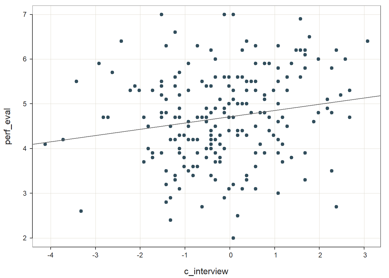
## >>> Suggestion
## # Create an R markdown file for interpretative output with Rmd = "file_name"
## reg(perf_eval ~ c_interview, data=DiffPred, rows=(race == "black" | race == "white"), Rmd="eg")
##
##
## BACKGROUND
##
## Data Frame: DiffPred
##
## Response Variable: perf_eval
## Predictor Variable: c_interview
##
## Number of cases (rows) of data: 212
## Number of cases retained for analysis: 212
##
##
## BASIC ANALYSIS
##
## Estimate Std Err t-value p-value Lower 95% Upper 95%
## (Intercept) 4.715 0.068 69.164 0.000 4.580 4.849
## c_interview 0.140 0.052 2.672 0.008 0.037 0.243
##
## Standard deviation of perf_eval: 1.004
##
## Standard deviation of residuals: 0.989 for 210 degrees of freedom
## 95% range of residual variation: 3.901 = 2 * (1.971 * 0.989)
##
## R-squared: 0.033 Adjusted R-squared: 0.028 PRESS R-squared: 0.014
##
## Null hypothesis of all 0 population slope coefficients:
## F-statistic: 7.139 df: 1 and 210 p-value: 0.008
##
## -- Analysis of Variance
##
## df Sum Sq Mean Sq F-value p-value
## Model 1 6.990 6.990 7.139 0.008
## Residuals 210 205.600 0.979
## perf_eval 211 212.590 1.008
##
##
## K-FOLD CROSS-VALIDATION
##
##
## RELATIONS AMONG THE VARIABLES
##
##
## RESIDUALS AND INFLUENCE
##
##
## PREDICTION ERRORWe should begin by noting that our effective sample size is now 212, whereas previously it was 370 when we included individuals of all races. The regression coefficient for c_interview is statistically significant and positive (b = .140, p = .008) based on this reduced sample of 212 individuals, which provides evidence of criterion-related validity. The amount of variance explained by c_interview in perf_eval is small in magnitude (R2 = .033, adjusted R2 = .028, p < .001).
Step Two: We will regress the criterion variable perf_eval on the selection tool variable c_interview and the protected class variable race.
# Regress perf_eval (criterion) on c_interview (selection tool) and protected class (race)
reg_brief(perf_eval ~ c_interview + race, data=DiffPred,
rows=(race=="black" | race=="white"))##
## >>> race is not numeric. Converted to indicator variables.
## >>> Suggestion
## # Create an R markdown file for interpretative output with Rmd = "file_name"
## reg(perf_eval ~ c_interview + race, data=DiffPred, rows=(race == "black" | race == "white"), Rmd="eg")
##
##
## BACKGROUND
##
## Data Frame: DiffPred
##
## Response Variable: perf_eval
## Predictor Variable 1: c_interview
## Predictor Variable 2: racewhite
##
## Number of cases (rows) of data: 212
## Number of cases retained for analysis: 212
##
##
## BASIC ANALYSIS
##
## Estimate Std Err t-value p-value Lower 95% Upper 95%
## (Intercept) 4.911 0.089 54.922 0.000 4.735 5.087
## c_interview 0.127 0.051 2.469 0.014 0.026 0.228
## racewhite -0.440 0.134 -3.287 0.001 -0.705 -0.176
##
## Standard deviation of perf_eval: 1.004
##
## Standard deviation of residuals: 0.967 for 209 degrees of freedom
## 95% range of residual variation: 3.813 = 2 * (1.971 * 0.967)
##
## R-squared: 0.080 Adjusted R-squared: 0.072 PRESS R-squared: NA
##
## Null hypothesis of all 0 population slope coefficients:
## F-statistic: 9.139 df: 2 and 209 p-value: 0.000
##
## -- Analysis of Variance from Type II Sums of Squares
##
## df Sum Sq Mean Sq F-value p-value
## c_interview 1 5.700 5.700 6.094 0.014
## racewhite 1 10.107 10.107 10.806 0.001
## Residuals 209 195.493 0.935
##
## -- Test of Interaction
##
## c_interview:race df: 1 df resid: 208 SS: 3.343 F: 3.618 p-value: 0.059
##
## -- Assume parallel lines, no interaction of race with c_interview
##
## Level black: y^_perf_eval = 4.911 + 0.127(x_c_interview)
## Level white: y^_perf_eval = 4.470 + 0.127(x_c_interview)
##
## -- Visualize Separately Computed Regression Lines
##
## Plot(c_interview, perf_eval, by=race, fit="lm")
##
##
## K-FOLD CROSS-VALIDATION
##
##
## RELATIONS AMONG THE VARIABLES
##
##
## RESIDUALS AND INFLUENCE
##
##
## PREDICTION ERRORThe regression coefficient associated with race (or more specifically racewhite) is negative and statistically significant (b = -.440, p = .001) when controlling for c_interview, which indicates that there is evidence of intercept differences. Because the coefficient is negative and because white is appended to the race variable name, it implies that the intercept value is significantly lower for White individuals compared to Black individuals. The amount of variance explained by c_interview and race in perf_eval is small-medium in magnitude (R2 = .080, adjusted R2 = .072, p < .001).
Using the probe_interaction function from the interactions package, we will visualize the intercept differences. As input to the probe_interaction function, use the lm function base R to specify our regression model from above. The subset= argument functions the same way as the rows= argument from the reg_brief and Regression functions from lessR, so we’ll use that instead for the lm function. Name this model something so that we can reference it in the next function (Int_Model).
# Regress perf_eval (criterion) on c_interview (selection tool) and protected class (race)
Int_Model <- lm(perf_eval ~ c_interview + race, data=DiffPred,
subset=(race=="black" | race=="white"))Let’s specify the arguments in the probe_interaction function to plot the intercept differences.
# Visualize intercept differences
probe_interaction(Int_Model,
pred=c_interview,
modx=race,
johnson_neyman=FALSE,
x.label="Interview Score",
y.label="Job Performance")## SIMPLE SLOPES ANALYSIS
##
## Slope of c_interview when race = white:
##
## Est. S.E. t val. p
## ------ ------ -------- ------
## 0.13 0.05 2.47 0.01
##
## Slope of c_interview when race = black:
##
## Est. S.E. t val. p
## ------ ------ -------- ------
## 0.13 0.05 2.47 0.01
Step Three: Finally, let’s add the interaction term between c_interview and race to the model using the * operator.
# Regress perf_eval (criterion) on c_interview (selection tool), protected class (race),
# and interaction between selection tool and protected class
reg_brief(perf_eval ~ c_interview * race, data=DiffPred,
rows=(race=="black" | race=="white"))##
## >>> race is not numeric. Converted to indicator variables.
## >>> Suggestion
## # Create an R markdown file for interpretative output with Rmd = "file_name"
## reg(perf_eval ~ c_interview * race, data=DiffPred, rows=(race == "black" | race == "white"), Rmd="eg")
##
##
## BACKGROUND
##
## Data Frame: DiffPred
##
## Response Variable: perf_eval
## Predictor Variable 1: c_interview
## Predictor Variable 2: racewhite
## Predictor Variable 3: c_interview.racewhite
##
## Number of cases (rows) of data: 212
## Number of cases retained for analysis: 212
##
##
## BASIC ANALYSIS
##
## Estimate Std Err t-value p-value Lower 95% Upper 95%
## (Intercept) 4.912 0.089 55.275 0.000 4.737 5.087
## c_interview 0.218 0.070 3.112 0.002 0.080 0.357
## racewhite -0.463 0.134 -3.466 0.001 -0.727 -0.200
## c_interview.racewhite -0.194 0.102 -1.902 0.059 -0.396 0.007
##
## Standard deviation of perf_eval: 1.004
##
## Standard deviation of residuals: 0.961 for 208 degrees of freedom
## 95% range of residual variation: 3.790 = 2 * (1.971 * 0.961)
##
## R-squared: 0.096 Adjusted R-squared: 0.083 PRESS R-squared: NA
##
## Null hypothesis of all 0 population slope coefficients:
## F-statistic: 7.375 df: 3 and 208 p-value: 0.000
##
## -- Analysis of Variance from Type II Sums of Squares
##
## df Sum Sq Mean Sq F-value p-value
## c_interview 1 5.700 5.700 6.094 0.014
## racewhite 1 10.107 10.107 10.941 0.001
## c_interview.racewhite 1 3.343 3.343 3.618 0.059
## Residuals 208 192.150 0.924
##
## -- Test of Interaction
##
## c_interview:race df: 1 df resid: 208 SS: 3.343 F: 3.618 p-value: 0.059
##
## -- Assume parallel lines, no interaction of race with c_interview
##
## Level black: y^_perf_eval = 4.912 + 0.218(x_c_interview)
## Level white: y^_perf_eval = 4.448 + 0.218(x_c_interview)
##
## -- Visualize Separately Computed Regression Lines
##
## Plot(c_interview, perf_eval, by=race, fit="lm")
##
##
## K-FOLD CROSS-VALIDATION
##
##
## RELATIONS AMONG THE VARIABLES
##
##
## RESIDUALS AND INFLUENCE
##
##
## PREDICTION ERRORThe regression coefficient associated with the interaction term (c_interview:racewhite) is not statistically significant (b = -.194, p = .059), which indicates that there is no evidence of slope differences. Given this, we won’t probe the interaction because, well, there is not an interaction to probe.
In sum, we found evidence of intercept differences for the selection tool c_interview in relation to the criterion perf_eval that were conditional upon the protected class variable race. Thus, it would be inappropriate to use a common regression line when predicting scores on the criterion based on the interview selection tool.
43.2.6 Summary
In this chapter, we learned how to use moderated multiple linear regression (MMLR) to test whether evidence of differential prediction exists. To do so, we learned how to use the Regression function (well, technically we used the reg_brief function) from lessR. In addition, we used the probe_interaction function from the interactions package to probe the intercept differences and slope differences visually and using simple slopes analyses.
43.3 Chapter Supplement
In addition to the Regression function from the lessR package covered above, we can use the lm function from base R to estimate a moderated multiple linear regression (MMLR) model. Because this function comes from base R, we do not need to install and access an additional package. In this supplement, you will also have an opportunity to learn how to make an APA (American Psychological Association) style table of regression results.
43.3.1 Functions & Packages Introduced
| Function | Package |
|---|---|
mean |
base R |
lm |
base R |
summary |
base R |
anova |
base R |
probe_interaction |
interactions |
apa.reg.table |
apaTables |
43.3.2 Initial Steps
If required, please refer to the Initial Steps section from this chapter for more information on these initial steps.
# Install readr package if you haven't already
# [Note: You don't need to install a package every
# time you wish to access it]
install.packages("readr")# Access readr package
library(readr)
# Read data and name data frame (tibble) object
DiffPred <- read_csv("DifferentialPrediction.csv")## Rows: 320 Columns: 6
## ── Column specification ────────────────────────────────────────────────────────────────────────────────────────────────────────────
## Delimiter: ","
## chr (3): emp_id, gender, race
## dbl (3): perf_eval, interview, age
##
## ℹ Use `spec()` to retrieve the full column specification for this data.
## ℹ Specify the column types or set `show_col_types = FALSE` to quiet this message.## [1] "emp_id" "perf_eval" "interview" "gender" "age" "race"## spc_tbl_ [320 × 6] (S3: spec_tbl_df/tbl_df/tbl/data.frame)
## $ emp_id : chr [1:320] "EE200" "EE202" "EE203" "EE206" ...
## $ perf_eval: num [1:320] 6.2 6.6 5 4 5.3 5.9 5.5 3.8 5.7 3.8 ...
## $ interview: num [1:320] 8.5 5.7 7 6.8 9.6 6 7.5 5.9 9.6 8.3 ...
## $ gender : chr [1:320] "woman" "woman" "man" "woman" ...
## $ age : num [1:320] 30 45.6 39.2 36.9 24.5 41.5 35.1 43.2 25.7 27.8 ...
## $ race : chr [1:320] "black" "black" "asian" "black" ...
## - attr(*, "spec")=
## .. cols(
## .. emp_id = col_character(),
## .. perf_eval = col_double(),
## .. interview = col_double(),
## .. gender = col_character(),
## .. age = col_double(),
## .. race = col_character()
## .. )
## - attr(*, "problems")=<externalptr>## # A tibble: 6 × 6
## emp_id perf_eval interview gender age race
## <chr> <dbl> <dbl> <chr> <dbl> <chr>
## 1 EE200 6.2 8.5 woman 30 black
## 2 EE202 6.6 5.7 woman 45.6 black
## 3 EE203 5 7 man 39.2 asian
## 4 EE206 4 6.8 woman 36.9 black
## 5 EE209 5.3 9.6 woman 24.5 white
## 6 EE214 5.9 6 woman 41.5 asian43.3.3 lm Function from Base R
We will use the lm function from base R to specify and estimate our regression functions. As I did above, I will show you how to apply moderated multiple linear regression (MMLR) in the service of detecting differential prediction of a selection tool based on protected class membership.
Grand-Mean Center Variables: Before we estimate the regression models, however, we need to grand-mean center certain variables. We only center predictor and moderator variables that are of type numeric and that we conceptualize as having a continuous (interval or ratio) measurement scale. In our current data frame, we will grand-mean center just the interview and age variables. We will use what is perhaps the most intuitive approach for grand-mean centering variables. We must begin by coming up with a new name for one of our soon-to-be grand-mean centered variable, and in this example, we will center the interview variable. I typically like to name the centered variable by simply adding the c_ prefix to the existing variable’s names (e.g., c_interview). Type the name of the data frame object to which the new centered variable will be attached (DiffPred), followed by the $ operator and the name of the new variable we are creating (c_interview). Next, add the <- operator to indicate what values you will assign to this new variable. To create a vector of values to assign to this new c_interview variable, we will subtract the mean (average) score for the original variable (interview) from each case’s value on the variable. Specifically, enter the name of the data frame object, followed by the $ operator and the name of the original variable (interview). After that, enter the subtraction operator (-). And finally, type the name of the mean function from base R. As the first argument in the mean function, enter the name of the data frame object (DiffPred), followed by the $ operator and the name of the original variable (interview). As the second argument, enter na.rm=TRUE to indicate that you wish to drop missing values when calculating the grand mean for the sample. Now repeat those same steps for the age variable.
# Grand-mean centering: Using basic arithmetic and the mean function from base R
DiffPred$c_interview <- DiffPred$interview - mean(DiffPred$interview, na.rm=TRUE)
DiffPred$c_age <- DiffPred$age - mean(DiffPred$age, na.rm=TRUE)43.3.3.1 Test Differential Prediction Based on gender
Let’s start with investigating whether differential prediction exists for our interview selection tool in relation to perf_eval based gender subgroup membership (i.e., man, woman).
Step One: Let’s being by regressing the criterion variable perf_eval on the selection tool variable c_interview. Here we are just establishing whether the selection tool shows evidence of criterion-related validity. See the chapters on criterion-related validity using correlation and predicting criterion scores using simple linear regression if you would like more information on regression-based approaches to assessing criterion-related validity, including determining whether statistical assumptions have been met. Let’s name our regression model for this first step model.1. Remember, we need to use the summary function from base R to view our model output.
# Regress perf_eval (criterion) on c_interview (selection tool)
model.1 <- lm(perf_eval ~ c_interview, data=DiffPred)
summary(model.1)##
## Call:
## lm(formula = perf_eval ~ c_interview, data = DiffPred)
##
## Residuals:
## Min 1Q Median 3Q Max
## -2.7226 -0.6846 0.0007 0.7494 2.5842
##
## Coefficients:
## Estimate Std. Error t value Pr(>|t|)
## (Intercept) 4.70750 0.05444 86.472 < 0.0000000000000002 ***
## c_interview 0.19175 0.04143 4.629 0.00000537 ***
## ---
## Signif. codes: 0 '***' 0.001 '**' 0.01 '*' 0.05 '.' 0.1 ' ' 1
##
## Residual standard error: 0.9738 on 318 degrees of freedom
## Multiple R-squared: 0.06312, Adjusted R-squared: 0.06018
## F-statistic: 21.43 on 1 and 318 DF, p-value: 0.000005366The regression coefficient for c_interview is statistically significant and positive (b = .192, p < .001), which provides evidence of criterion-related validity. The amount of variance explained by c_interview in perf_eval is small-medium in magnitude (R2 = .063, adjusted R2 = .060, p < .001). See the table below for common rules of thumbs for qualitatively describing R2 values.
| R2 | Description |
|---|---|
| .01 | Small |
| .09 | Medium |
| .25 | Large |
Step Two: Next, let’s add the protected class variable gender to our model to investigate whether intercept differences exist. We’ll name this model model.2. For more information on how to interpret and test the statistical assumptions of a multiple linear regression model, check out the chapter on estimating incremental validity. In addition, let’s use the anova function from base R to do a nested model comparison between model.1 and model.2. This will tell us whether adding gender to the model significantly improved model fit. Finally, let’s reference the summary/output for each model and specifically the r.squared values to determine what the change in R2 was from one model to the next. The change in R2 gives as an idea of how much (in terms of practical significance) the model fit improved when adding the additional variable. Note that we use the $ operator to indicate that we want the r.squared value from the summary(model.2) and summary(model.2) output, and then we do a simple subtraction to get the change in R2.
# Regress perf_eval (criterion) on c_interview (selection tool) and protected class (gender)
model.2 <- lm(perf_eval ~ c_interview + gender, data=DiffPred)
summary(model.2)##
## Call:
## lm(formula = perf_eval ~ c_interview + gender, data = DiffPred)
##
## Residuals:
## Min 1Q Median 3Q Max
## -2.8125 -0.6629 0.0049 0.7578 2.5245
##
## Coefficients:
## Estimate Std. Error t value Pr(>|t|)
## (Intercept) 4.62953 0.07625 60.719 < 0.0000000000000002 ***
## c_interview 0.21058 0.04332 4.861 0.00000184 ***
## genderwoman 0.16634 0.11409 1.458 0.146
## ---
## Signif. codes: 0 '***' 0.001 '**' 0.01 '*' 0.05 '.' 0.1 ' ' 1
##
## Residual standard error: 0.9721 on 317 degrees of freedom
## Multiple R-squared: 0.06936, Adjusted R-squared: 0.06349
## F-statistic: 11.81 on 2 and 317 DF, p-value: 0.00001127## Analysis of Variance Table
##
## Model 1: perf_eval ~ c_interview
## Model 2: perf_eval ~ c_interview + gender
## Res.Df RSS Df Sum of Sq F Pr(>F)
## 1 318 301.58
## 2 317 299.57 1 2.0086 2.1255 0.1459## [1] 0.006239901The unstandardized regression coefficient associated with gender (or more specifically genderwoman) is not statistically significant (b = .166, p = .146) when controlling for c_interview, which indicates that there is no evidence of intercept differences. Note that the name of the regression coefficient for gender has woman appended to it; this means that the intercept represents the perf_eval scores of women minus those for men. Behind the scenes, the reg_brief function has converted the gender variable to a dichotomous factor, where alphabetically man becomes 0 and woman becomes 1. Because the coefficient is negative, it implies that the intercept value is higher for women relative to men; however, please note that we wouldn’t interpret the direction of this effect because it was not statistically significant. The amount of variance explained by c_interview and gender in perf_eval is small-medium in magnitude (R2 = .069, adjusted R2 = .063, p < .001), which is slightly larger than when just c_interview was included in the model (see Step One above). The nonsignificant F-value (2.126, p = .146) in from the nested model comparison indicates that adding gender to the model did not significantly improve model fit, and thus we will not interpret the change in R2.
Because there is no evidence of intercept differences for Step Two, we won’t plot/graph the our model, as doing so might mislead someone who sees such a plot without knowing or understanding the results of the model we just estimated. We will now proceed to Step Three.
Step Three: As the final step, it’s time to add the interaction term (also known as a product term) between c_interview and gender to the model, which creates what is referred to as a multiplicative model. Fortunately, this is very easy to do in R. All we need to do is change the + operator from our previous regression model script to the *, where the * implies an interaction in the context of a model. Conceptually, the * is appropriate because we are estimating a multiplicative model containing an interaction term. Let’s name this model model.3. As before, we’ll do a nested model comparison between the previous model and this model to determine whether there is a significant improvement in model fit. In addition, we’ll estimate change in R2.
# Regress perf_eval (criterion) on c_interview (selection tool), protected class (gender),
# and interaction between selection tool and protected class
model.3 <- lm(perf_eval ~ c_interview * gender, data=DiffPred)
summary(model.3)##
## Call:
## lm(formula = perf_eval ~ c_interview * gender, data = DiffPred)
##
## Residuals:
## Min 1Q Median 3Q Max
## -2.71851 -0.67772 0.01742 0.69477 2.48590
##
## Coefficients:
## Estimate Std. Error t value Pr(>|t|)
## (Intercept) 4.56191 0.07566 60.298 < 0.0000000000000002 ***
## c_interview 0.39426 0.05909 6.672 0.000000000113 ***
## genderwoman 0.15494 0.11091 1.397 0.163
## c_interview:genderwoman -0.37306 0.08422 -4.430 0.000013026266 ***
## ---
## Signif. codes: 0 '***' 0.001 '**' 0.01 '*' 0.05 '.' 0.1 ' ' 1
##
## Residual standard error: 0.9448 on 316 degrees of freedom
## Multiple R-squared: 0.1238, Adjusted R-squared: 0.1155
## F-statistic: 14.88 on 3 and 316 DF, p-value: 0.000000004387## Analysis of Variance Table
##
## Model 1: perf_eval ~ c_interview + gender
## Model 2: perf_eval ~ c_interview * gender
## Res.Df RSS Df Sum of Sq F Pr(>F)
## 1 317 299.57
## 2 316 282.06 1 17.514 19.622 0.00001303 ***
## ---
## Signif. codes: 0 '***' 0.001 '**' 0.01 '*' 0.05 '.' 0.1 ' ' 1## [1] 0.05440861In our output, we now have an unstandardized regression coefficient called c_interview:gender (or c_interview.gender), which represents our interaction term for c_interview and gender. The regression coefficient associated with the interaction term (c_interview:gender) is negative and statistically significant (b = -.373, p < .001), but we shouldn’t pay too much attention to the sign of the interaction term as it is difficult to interpret it without graphing the regression model in its entirety. We should, however, pay attention to the fact that the interaction term is statistically significant, which indicates that there is evidence of slope differences; in other words, there seems to be multiplicative effect between c_interview and gender. Although we didn’t find evidence of intercept differences in Step Two, here in Step Three, we do find evidence that the criterion-related validities for the selection tool (c_interview) in relation to the criterion (perf_eval) are significantly different from one another; in other words, we found evidence that the slopes for men and women differ. The amount of variance explained by c_interview, gender, and their interaction in relation to perf_eval is medium in magnitude (R2 = .124, adjusted R2 = .115, p < .001), which is larger than when just c_interview and gender were included in the model (see Step Two above). The significant F-value (19.622, p < .001) in from the nested model comparison indicates that adding the interaction term significantly improved model fit, and because there was a significant improvement in model fit, we should interpret the change in R2 (R2 = .054), which indicates that adding the interaction term to the model explained an additional 5.4% of the variance in perf_eval.
Given the statistically significant interaction term, it is appropriate (and helpful) to probe the interaction by plotting it. This will help us understand the form of the interaction. We can do so by creating a plot of the simple slopes. To do so, we will use a package called interactions (Long 2019), so if you haven’t already, install and access the package.
# Install interactions package if you haven't already
install.packages("interactions")

# Note: You may need to install the sandwich package independently if you
# receive an error when attempting to run the probe_interaction function
# install.packages("sandwich")As the first argument in the probe_interaction function from the interactions package, enter the name of the regression model we just created above (model.3). As the second argument, type the name of the variable you are framing as the predictor after pred=, which in our case is the selection tool variable (c_interview). As the third argument, type the name of the variable you are framing as the moderator after modx=, which in our case is the protected class variable (gender). As the fourth argument, enter johnson_neyman=FALSE, as we aren’t requesting the Johnson-Neyman test in this tutorial. Finally, if you choose to, you can use x.label= and y.label= to create more informative names for the predictor and outcome variables, respectively. You could also add, if you should choose to do so, the legend.main= argument to provide a more informative name for the moderator variable, and/or the modx.labels= to provide more informative names for the moderator variable labels.
# Probe the significant interaction (slope differences)
probe_interaction(model.3,
pred=c_interview,
modx=gender,
johnson_neyman=FALSE,
x.label="Interview Score",
y.label="Job Performance")## SIMPLE SLOPES ANALYSIS
##
## Slope of c_interview when gender = man:
##
## Est. S.E. t val. p
## ------ ------ -------- ------
## 0.39 0.06 6.67 0.00
##
## Slope of c_interview when gender = woman:
##
## Est. S.E. t val. p
## ------ ------ -------- ------
## 0.02 0.06 0.35 0.72
The plot output shows that the two slopes are indeed different, such that there doesn’t seem to be much of an association between the selection tool (c_interview) and the criterion (perf_eval) for women, but there seems to be a positive association for men. Now take a look at the text output in your console. The simple slopes analysis automatically estimates the regression coefficient (slope) for both levels of the moderator variable (gender: man, woman). Corroborating what we see in the plot, we find that the simple slope for men is indeed statistically significant and positive (b = .39, p < .01), such that for every one unit increase in interview scores, job performance scores tend to go up by .39 units. In contrast, we find that the simple slope for women is nonsignificant (b = .02, p = .72).
In sum, we found evidence of slope differences – but not intercept differences – for the selection tool (c_interview) in relation to the criterion (perf_eval) that were conditional upon the levels/subgroups of the protected class variable (gender). Thus, we can conclude that there is evidence of differential prediction based on gender for this interview selection tool, which means that it would be inappropriate to use a common regression line when predicting scores on the criterion based on the interview selection tool.
Sample Write-Up: Our HR analytics team recently found evidence in support of the criterion-related validity of a new structured interview selection procedure. As a next step, we investigated whether there might be evidence of differential prediction of the structured interview based on the U.S. protected class of gender. Based on a sample of 370 individuals, we applied a three-step process with moderated multiple linear regression, which is consistent with established principles (Society for Industrial & Organizational Psychology 2018; Cleary 1968). Based on our analyses, we found evidence differential prediction (i.e., predictive bias) based on gender for the new structured interview procedure, and specifically, we found evidence of slope differences. In the first step, we found evidence of criterion-related validity based on a simple linear regression model, as structured interview scores were positively and significantly associated with job performance (b = .192, p < .001), thereby indicating some degree of job-relatedness and -relevance. In the second step, we added the protected class variable associated with gender to the model, resulting in a multiple linear regression model, but did not find evidence of intercept differences based on gender (b = .166, p = .146). In the third step, we added the interaction term between the structured interview and gender variables, resulting in a moderated multiple linear regression model, and we found that gender moderated the association between structured interview scores and job performance scores to a statistically significant extent (b = -.373, p < .001). Based on follow-up simple slopes analyses, we found that the association between structured interview scores and job performance scores was statistically significant for men (b = .39, p < .01), such that for every one unit increase in structured interview scores, job performance scores tended to increase by .39 units; in contrast, the associated between structured interview scores and job performance scores for women was nonsignificant (b = .02, p = .72). In sum, we found evidence slope differences, which means that this structured interview tool shows predictive bias with respect to gender, making the application of a common regression line (i.e., equation) legally problematic within the United States. If possible, this structured interview should be redesigned or the interviewers should be trained to reduce the predictive bias based on gender. In the interim, we caution against using separate regression lines for men and women, as this may be interpreted as running afoul of the U.S. Civil Rights Act of 1991 (Saad and Sackett 2002). A more conservative approach would be to develop a structured interview process that allows for the use of a common regression line across legally protected groups.
43.3.3.2 Test Differential Prediction Based on c_age
Investigating whether differential prediction exists for c_interview in relation to perf_eval based on the continuous moderator variable c_age will unfold very similarly to the process we used for the dichotomous gender variable from above. The only differences will occur when it comes to estimating and visualizing the intercept differences and simple slopes (assuming we find statistically significant effects). Given this, we will breeze through the steps, which means I will provide less explanation.
Step One: Regress the criterion variable perf_eval on the selection tool variable c_interview.
# Regress perf_eval (criterion) on c_interview (selection tool)
model.1 <- lm(perf_eval ~ c_interview, data=DiffPred)
summary(model.1)
##
## Call:
## lm(formula = perf_eval ~ c_interview, data = DiffPred)
##
## Residuals:
## Min 1Q Median 3Q Max
## -2.7226 -0.6846 0.0007 0.7494 2.5842
##
## Coefficients:
## Estimate Std. Error t value Pr(>|t|)
## (Intercept) 4.70750 0.05444 86.472 < 0.0000000000000002 ***
## c_interview 0.19175 0.04143 4.629 0.00000537 ***
## ---
## Signif. codes: 0 '***' 0.001 '**' 0.01 '*' 0.05 '.' 0.1 ' ' 1
##
## Residual standard error: 0.9738 on 318 degrees of freedom
## Multiple R-squared: 0.06312, Adjusted R-squared: 0.06018
## F-statistic: 21.43 on 1 and 318 DF, p-value: 0.000005366The regression coefficient for c_interview is statistically significant and positive (b = .192, p < .001), which provides evidence of criterion-related validity. The amount of variance explained by c_interview in perf_eval is small-medium in magnitude (R2 = .063, adjusted R2 = .060, p < .001).
Step Two: Regress the criterion variable perf_eval on the selection tool variable c_interview and the protected class variable c_age. In addition, do a nested model comparison, and estimate the change in R2.
# Regress perf_eval (criterion) on c_interview (selection tool) and protected class (c_age)
model.2 <- lm(perf_eval ~ c_interview + c_age, data=DiffPred)
summary(model.2)
##
## Call:
## lm(formula = perf_eval ~ c_interview + c_age, data = DiffPred)
##
## Residuals:
## Min 1Q Median 3Q Max
## -3.2596 -0.6087 0.0444 0.6184 2.5522
##
## Coefficients:
## Estimate Std. Error t value Pr(>|t|)
## (Intercept) 4.70750 0.04999 94.164 < 0.0000000000000002 ***
## c_interview 0.97806 0.10833 9.028 < 0.0000000000000002 ***
## c_age 0.12863 0.01659 7.752 0.000000000000124 ***
## ---
## Signif. codes: 0 '***' 0.001 '**' 0.01 '*' 0.05 '.' 0.1 ' ' 1
##
## Residual standard error: 0.8943 on 317 degrees of freedom
## Multiple R-squared: 0.2124, Adjusted R-squared: 0.2075
## F-statistic: 42.75 on 2 and 317 DF, p-value: < 0.00000000000000022## Analysis of Variance Table
##
## Model 1: perf_eval ~ c_interview
## Model 2: perf_eval ~ c_interview + c_age
## Res.Df RSS Df Sum of Sq F Pr(>F)
## 1 318 301.58
## 2 317 253.52 1 48.059 60.092 0.0000000000001241 ***
## ---
## Signif. codes: 0 '***' 0.001 '**' 0.01 '*' 0.05 '.' 0.1 ' ' 1## [1] 0.1492979The regression coefficient associated with c_age is positive and statistically significant (b = .129, p < .001) when controlling for c_interview, which indicates that there is evidence of intercept differences. Because the coefficient is positive, it implies that the intercept value is significantly higher for older workers relative to younger workers. The amount of variance explained by c_interview and c_age in perf_eval is medium-large in magnitude (R2 = .212, adjusted R2 = .207, p < .001), which is notably larger than when just c_interview was included in the model (see Step One above). The significant F-value (60.092, p < .001) in from the nested model comparison indicates that adding c_age significantly improved model fit, and because there was a significant improvement in model fit, we should interpret the change in R2 (R2 = .149), which indicates that adding c_age to the model explained an additional 14.9% of the variance in perf_eval.
Using the probe_interaction function from the interactions package, we will visualize the intercept differences of the model.2 model we specified above. Note that the function automatically categorizes the continuous moderator variable by its mean and 1 standard deviation (SD) below and above the mean. As you can see in the plot, individuals whose age is 1 SD above the mean have the highest intercept value, where the intercept is the value of perf_eval (Job Performance) when interview (Interview) is equal to zero.
# Visualize intercept differences
probe_interaction(model.2,
                  pred=c_interview,
                  modx=c_age,
                  johnson_neyman=FALSE,
                  x.label="Interview Score",
                  y.label="Job Performance")
## SIMPLE SLOPES ANALYSIS
##
## Slope of c_interview when c_age = -8.593122204199181268791 (- 1 SD):
##
## Est. S.E. t val. p
## ------ ------ -------- ------
## 0.98 0.11 9.03 0.00
##
## Slope of c_interview when c_age = -0.000000000000003164136 (Mean):
##
## Est. S.E. t val. p
## ------ ------ -------- ------
## 0.98 0.11 9.03 0.00
##
## Slope of c_interview when c_age = 8.593122204199174163364 (+ 1 SD):
##
## Est. S.E. t val. p
## ------ ------ -------- ------
## 0.98 0.11 9.03 0.00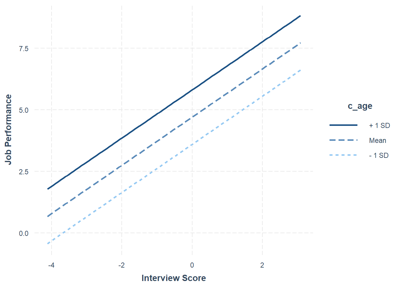
Step Three: Now, we will add the interaction term between c_interview and c_age to the model using the * operator. In addition, do a nested model comparison, and estimate the change in R2.
# Regress perf_eval (criterion) on c_interview (selection tool) and protected class (c_age)
model.3 <- lm(perf_eval ~ c_interview * c_age, data=DiffPred)
summary(model.3)
##
## Call:
## lm(formula = perf_eval ~ c_interview * c_age, data = DiffPred)
##
## Residuals:
## Min 1Q Median 3Q Max
## -3.6271 -0.5798 0.0261 0.5553 2.4924
##
## Coefficients:
## Estimate Std. Error t value Pr(>|t|)
## (Intercept) 4.995359 0.067563 73.937 < 0.0000000000000002 ***
## c_interview 1.711274 0.159937 10.700 < 0.0000000000000002 ***
## c_age 0.263061 0.027431 9.590 < 0.0000000000000002 ***
## c_interview:c_age 0.027267 0.004555 5.986 0.00000000585 ***
## ---
## Signif. codes: 0 '***' 0.001 '**' 0.01 '*' 0.05 '.' 0.1 ' ' 1
##
## Residual standard error: 0.8489 on 316 degrees of freedom
## Multiple R-squared: 0.2926, Adjusted R-squared: 0.2859
## F-statistic: 43.57 on 3 and 316 DF, p-value: < 0.00000000000000022## Analysis of Variance Table
##
## Model 1: perf_eval ~ c_interview + c_age
## Model 2: perf_eval ~ c_interview * c_age
## Res.Df RSS Df Sum of Sq F Pr(>F)
## 1 317 253.52
## 2 316 227.71 1 25.817 35.827 0.000000005849 ***
## ---
## Signif. codes: 0 '***' 0.001 '**' 0.01 '*' 0.05 '.' 0.1 ' ' 1## [1] 0.08020031The regression coefficient associated with the interaction term (c_interview:c_age) is positive and statistically significant (b = .027, p < .001), which indicates that there is evidence of slope differences. The amount of variance explained by c_interview, c_age, and their interaction in relation to perf_eval is large in magnitude (R2 = .293, adjusted R2 = .286, p < .001), which is larger than when just c_interview and c_age were included in the model. The significant F-value (35.827, p < .001) in from the nested model comparison indicates that adding the interaction term significantly improved model fit, and because there was a significant improvement in model fit, we should interpret the change in R2 (R2 = .080), which indicates that adding the interaction term to the model explained an additional 8.0% of the variance in perf_eval.
Given the statistically significant interaction term, we will use the probe_interaction function from the interactions package to probe the interaction to plot this multiplicative model that we named model.3.
# Probe the significant interaction (slope differences)
probe_interaction(model.3,
                  pred=c_interview,
                  modx=c_age,
                  johnson_neyman=FALSE,
                  x.label="Interview Score",
                  y.label="Job Performance")
## SIMPLE SLOPES ANALYSIS
##
## Slope of c_interview when c_age = -8.593122204199181268791 (- 1 SD):
##
## Est. S.E. t val. p
## ------ ------ -------- ------
## 1.48 0.13 11.16 0.00
##
## Slope of c_interview when c_age = -0.000000000000003164136 (Mean):
##
## Est. S.E. t val. p
## ------ ------ -------- ------
## 1.71 0.16 10.70 0.00
##
## Slope of c_interview when c_age = 8.593122204199174163364 (+ 1 SD):
##
## Est. S.E. t val. p
## ------ ------ -------- ------
## 1.95 0.19 10.16 0.00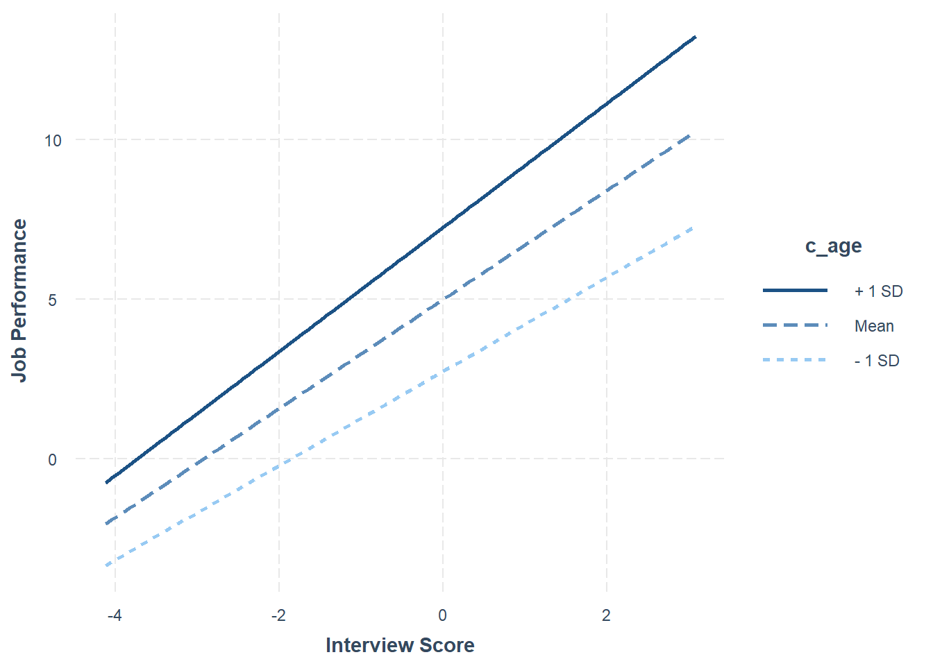
The plot and the simple slopes analyses output show that the two slopes are indeed different, such that the association between the selection tool (c_interview, Interview) and the criterion (perf_eval, Job Performance) is more positive for older workers (b = 1.95, p < .01), than for average-aged workers (b = 1.71, p < .01) and younger workers (b = 1.48, p < .01). Notably, all three simple slopes are statistically significant and positive, but the slope is more positive for older workers.
In sum, we found evidence of both intercept and slope differences for the selection tool (c_interview) in relation to the criterion (perf_eval) that were conditional upon the age protected class variable (c_age). Thus, it would be inappropriate to use a common regression line when predicting scores on the criterion based on the interview selection tool.
43.3.3.3 Test Differential Prediction Based on race
To investigate whether differential prediction exists for c_interview in relation to perf_eval based on race, we will follow mostly the same process as we did with the dichotomous variable gender above. However, we will filter our data within the regression function to compare just Black individuals with White individuals, as it is customary to compare just two races/ethnicities at a time. The decision to focus on only Black and White individuals is arbitrary and just for demonstration purposes. Note that in the DiffPred data frame object that both black and white are lowercase category labels in the race variable.
Step One: Regress the criterion variable perf_eval on the selection tool variable c_interview. Add the subset=(race=="black" | race=="white") argument to subset the data such that only those individuals who are Black and White are retained. In doing so, we effectively dichotomize the race variable within the lm function. If you need to review conditional/logical statements when filtering data, check out the chapter on filtering data.
# Regress perf_eval (criterion) on c_interview (selection tool)
model.1 <- lm(perf_eval ~ c_interview, data=DiffPred,
              subset=(race=="black" | race=="white"))
summary(model.1)
##
## Call:
## lm(formula = perf_eval ~ c_interview, data = DiffPred, subset = (race ==
## "black" | race == "white"))
##
## Residuals:
## Min 1Q Median 3Q Max
## -2.72580 -0.66775 -0.00208 0.74761 2.49792
##
## Coefficients:
## Estimate Std. Error t value Pr(>|t|)
## (Intercept) 4.71479 0.06817 69.164 < 0.0000000000000002 ***
## c_interview 0.13983 0.05233 2.672 0.00813 **
## ---
## Signif. codes: 0 '***' 0.001 '**' 0.01 '*' 0.05 '.' 0.1 ' ' 1
##
## Residual standard error: 0.9895 on 210 degrees of freedom
## Multiple R-squared: 0.03288, Adjusted R-squared: 0.02827
## F-statistic: 7.139 on 1 and 210 DF, p-value: 0.008133We should begin by noting that our effective sample size is now 212 (which we can compute by adding the number of degrees of freedom in our model, 212, to the number of parameters estimated, 2), whereas previously it was 370 when we included individuals of all races. The regression coefficient for c_interview is statistically significant and positive (b = .140, p = .008) based on this reduced sample of 212 individuals, which provides evidence of criterion-related validity. The amount of variance explained by c_interview in perf_eval is small in magnitude (R2 = .033, adjusted R2 = .028, p < .001).
Step Two: Regress the criterion variable perf_eval on the selection tool variable c_interview and the protected class variable race. In addition, do a nested model comparison, and estimate the change in R2.
# Regress perf_eval (criterion) on c_interview (selection tool) and protected class (race)
model.2 <- lm(perf_eval ~ c_interview + race, data=DiffPred,
              subset=(race=="black" | race=="white"))
summary(model.2)
##
## Call:
## lm(formula = perf_eval ~ c_interview + race, data = DiffPred,
## subset = (race == "black" | race == "white"))
##
## Residuals:
## Min 1Q Median 3Q Max
## -2.51207 -0.64712 -0.03035 0.65707 2.28188
##
## Coefficients:
## Estimate Std. Error t value Pr(>|t|)
## (Intercept) 4.91079 0.08941 54.922 < 0.0000000000000002 ***
## c_interview 0.12665 0.05131 2.469 0.01437 *
## racewhite -0.44041 0.13398 -3.287 0.00119 **
## ---
## Signif. codes: 0 '***' 0.001 '**' 0.01 '*' 0.05 '.' 0.1 ' ' 1
##
## Residual standard error: 0.9671 on 209 degrees of freedom
## Multiple R-squared: 0.08042, Adjusted R-squared: 0.07162
## F-statistic: 9.139 on 2 and 209 DF, p-value: 0.0001567## Analysis of Variance Table
##
## Model 1: perf_eval ~ c_interview
## Model 2: perf_eval ~ c_interview + race
## Res.Df RSS Df Sum of Sq F Pr(>F)
## 1 210 205.60
## 2 209 195.49 1 10.107 10.806 0.001187 **
## ---
## Signif. codes: 0 '***' 0.001 '**' 0.01 '*' 0.05 '.' 0.1 ' ' 1## [1] 0.04754406The regression coefficient associated with race (or more specifically racewhite) is negative and statistically significant (b = -.440, p = .001) when controlling for c_interview, which indicates that there is evidence of intercept differences. Because the coefficient is negative and because white is appended to the race variable name, it implies that the intercept value is significantly lower for White individuals compared to Black individuals. The amount of variance explained by c_interview and race in perf_eval is small-medium in magnitude (R2 = .080, adjusted R2 = .072, p < .001). The significant F-value (10.806, p = .001) from the nested model comparison indicates that adding race significantly improved model fit, and because there was a significant improvement in model fit, we should interpret the change in R2 (R2 = .048), which indicates that adding race to the model explained an additional 4.8% of the variance in perf_eval.
Using the probe_interaction function from the interactions package, we will visualize the statistically significant intercept differences. As input to the probe_interaction function, use the the model.2 model object from above, and specify the arguments in the probe_interaction function as you did before.
# Visualize intercept differences
probe_interaction(model.2,
                  pred=c_interview,
                  modx=race,
                  johnson_neyman=FALSE,
                  x.label="Interview Score",
                  y.label="Job Performance")
## SIMPLE SLOPES ANALYSIS
##
## Slope of c_interview when race = white:
##
## Est. S.E. t val. p
## ------ ------ -------- ------
## 0.13 0.05 2.47 0.01
##
## Slope of c_interview when race = black:
##
## Est. S.E. t val. p
## ------ ------ -------- ------
## 0.13 0.05 2.47 0.01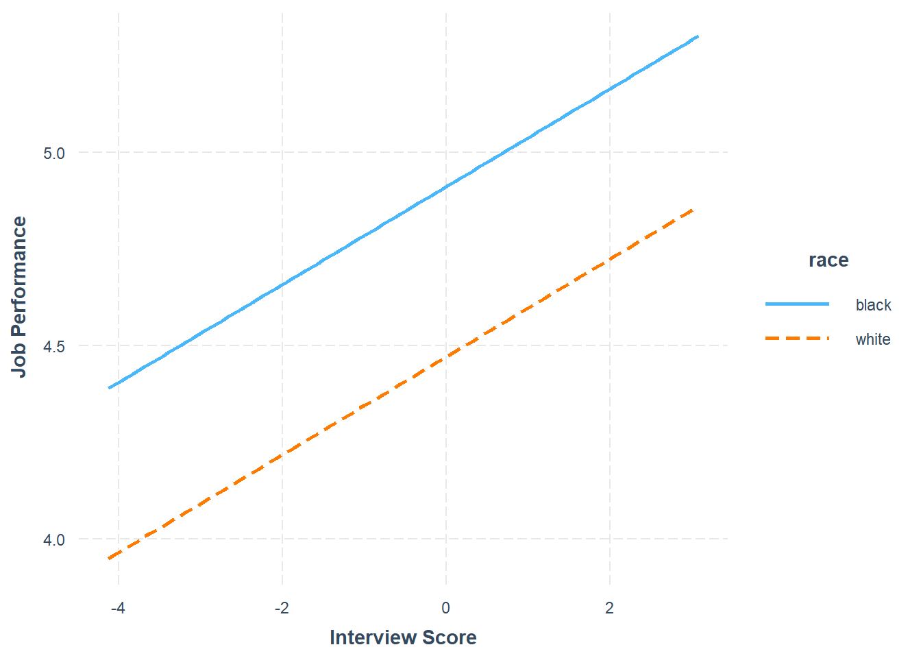
Step Three: Finally, let’s add the interaction term between c_interview and race to the model using the * operator. In addition, do a nested model comparison, and estimate the change in R2.
# Regress perf_eval (criterion) on c_interview (selection tool), protected class (race),
# and interaction between selection tool and protected class
model.3 <- lm(perf_eval ~ c_interview * race, data=DiffPred,
              subset=(race=="black" | race=="white"))
summary(model.3)
##
## Call:
## lm(formula = perf_eval ~ c_interview * race, data = DiffPred,
## subset = (race == "black" | race == "white"))
##
## Residuals:
## Min 1Q Median 3Q Max
## -2.7314 -0.6396 0.0227 0.6637 2.4205
##
## Coefficients:
## Estimate Std. Error t value Pr(>|t|)
## (Intercept) 4.91180 0.08886 55.275 < 0.0000000000000002 ***
## c_interview 0.21843 0.07020 3.112 0.002122 **
## racewhite -0.46345 0.13370 -3.466 0.000641 ***
## c_interview:racewhite -0.19428 0.10213 -1.902 0.058527 .
## ---
## Signif. codes: 0 '***' 0.001 '**' 0.01 '*' 0.05 '.' 0.1 ' ' 1
##
## Residual standard error: 0.9611 on 208 degrees of freedom
## Multiple R-squared: 0.09615, Adjusted R-squared: 0.08311
## F-statistic: 7.375 on 3 and 208 DF, p-value: 0.0001015## Analysis of Variance Table
##
## Model 1: perf_eval ~ c_interview + race
## Model 2: perf_eval ~ c_interview * race
## Res.Df RSS Df Sum of Sq F Pr(>F)
## 1 209 195.49
## 2 208 192.15 1 3.3426 3.6184 0.05853 .
## ---
## Signif. codes: 0 '***' 0.001 '**' 0.01 '*' 0.05 '.' 0.1 ' ' 1## [1] 0.0157234The regression coefficient associated with the interaction term (c_interview:racewhite) is not statistically significant (b = -.194, p = .059), which indicates that there is no evidence of slope differences. Given this, we won’t probe the interaction because, well, there is not an interaction to probe. Further, adding the interaction term did not significantly improve model fit, so we won’t interpret change in R2. Given all this, we won’t probe the interaction because, well, there is not an interaction to probe.
In sum, we found evidence of intercept differences for the selection tool c_interview in relation to the criterion perf_eval that were conditional upon the protected class variable race. Thus, it would be inappropriate to use a common regression line when predicting scores on the criterion based on the interview selection tool.
43.3.4 APA-Style Results Table
If you want to present the results of your moderated multiple linear regression (MMLR) model to a more statistically inclined audience, particularly an audience that prefers American Psychological Association (APA) style, consider using functions from the apaTables package (Stanley 2021).
Using the lm function from base R, as we did above, let’s begin by estimating a MMLR model and naming the model object (model.3).
# Estimate multiple linear regression model
model.3 <- lm(perf_eval ~ c_interview * gender, data=DiffPred)
If you haven’t already, install and access the apaTables package using the install.packages and library functions, respectively.
The apa.reg.table function from apaTables is pretty straightforward. Simply enter your regression model object (model.3) as the sole parenthetical argument. This will generate a table as output in your Console.
##
##
## Regression results using perf_eval as the criterion
##
##
##                Predictor       b       b_95%_CI sr2  sr2_95%_CI             Fit
##              (Intercept)  4.56**   [4.41, 4.71]
##              c_interview  0.39**   [0.28, 0.51] .12  [.06, .19]
##              genderwoman    0.15  [-0.06, 0.37] .01 [-.01, .02]
##  c_interview:genderwoman -0.37** [-0.54, -0.21] .05  [.01, .10]
##                                                                     R2 = .124**
##                                                                 95% CI[.06,.19]
##
##
## Note. A significant b-weight indicates the semi-partial correlation is also significant.
## b represents unstandardized regression weights.
## sr2 represents the semi-partial correlation squared.
## Square brackets are used to enclose the lower and upper limits of a confidence interval.
## * indicates p < .05. ** indicates p < .01.
##
If we add a filename= as a second argument, we can specify the name of a .doc file that we can write to our working directory. Here, I name the file “APA Multiple Linear Regression Table.doc”. The .doc file that appears in your working directory will be nicely formatted and include critical regression model results in an organized manner.
# Create APA-style regression table and write to working directory
apa.reg.table(model.3, filename="APA Moderated Multiple Linear Regression Table.doc")
##
##
## Regression results using perf_eval as the criterion
##
##
## Predictor b b_95%_CI sr2 sr2_95%_CI Fit
## (Intercept) 4.56** [4.41, 4.71]
## c_interview 0.39** [0.28, 0.51] .12 [.06, .19]
## genderwoman 0.15 [-0.06, 0.37] .01 [-.01, .02]
## c_interview:genderwoman -0.37** [-0.54, -0.21] .05 [.01, .10]
## R2 = .124**
## 95% CI[.06,.19]
##
##
## Note. A significant b-weight indicates the semi-partial correlation is also significant.
## b represents unstandardized regression weights.
## sr2 represents the semi-partial correlation squared.
## Square brackets are used to enclose the lower and upper limits of a confidence interval.
## * indicates p < .05. ** indicates p < .01.
##